Добавил:
Опубликованный материал нарушает ваши авторские права? Сообщите нам.
Вуз: Предмет: Файл:
[James_Stewart]_Single_Variable_Calculus_Early_Tr(BookFi).pdf
Скачиваний:
35
Добавлен:
30.12.2019
Размер:
18.09 Mб
Скачать

550 |||| CHAPTER 8 FURTHER APPLICATIONS OF INTEGRATION

D I S C O V E R Y

P R O J E C T

COMPLEMENTARY COFFEE CUPS

Suppose you have a choice of two coffee cups of the type shown, one that bends outward and one inward, and you notice that they have the same height and their shapes fit together snugly. You wonder which cup holds more coffee. Of course you could fill one cup with water and pour it into the other one but, being a calculus student, you decide on a more mathematical approach. Ignoring the handles, you observe that both cups are surfaces of revolution, so you can think of the coffee as a volume of revolution.


y

x=k


h


A™


x=f(y)


0

k

x

Cup A

Cup B


1.Suppose the cups have height h, cup A is formed by rotating the curve x f y about the y-axis, and cup B is formed by rotating the same curve about the line x k. Find the value of k such that the two cups hold the same amount of coffee.

2.What does your result from Problem 1 say about the areas A1 and A2 shown in the figure?

3.Use Pappus’s Theorem to explain your result in Problems 1 and 2.

4.Based on your own measurements and observations, suggest a value for h and an equation for x f y and calculate the amount of coffee that each cup holds.


8.4


APPLICATIONS TO ECONOMICS AND BIOLOGY


In this section we consider some applications of integration to economics (consumer sur-


plus) and biology (blood flow, cardiac output). Others are described in the exercises.


CONSUMER SURPLUS


p


Recall from Section 4.7 that the demand function p x is the price that a company has to


charge in order to sell x units of a commodity. Usually, selling larger quantities requires


p=p(x)


lowering prices, so the demand function is a decreasing function. The graph of a typical


demand function, called a demand curve, is shown in Figure 1. If X is the amount of the


commodity that is currently available, then P p X is the current selling price.


We divide the interval 0, X into n subintervals, each of length x X n, and let


P


(X,P)


xi* xi be the right endpoint of the ith subinterval, as in Figure 2. If, after the first xi 1


units were sold, a total of only xi units had been available and the price per unit had been


set at p xi dollars, then the additional x units could have been sold (but no more). The


0


X

x


consumers who would have paid p xi dollars placed a high value on the product; they


would have paid what it was worth to them. So, in paying only P dollars they have saved


FIGURE 1


an amount of

A typical demand curve

savings per unit number of units p xi P x

SECTION 8.4 APPLICATIONS TO ECONOMICS AND BIOLOGY |||| 551

p


Considering similar groups of willing consumers for each of the subintervals and adding


the savings, we get the total savings:


n


p xi P x


i 1


(X,P)


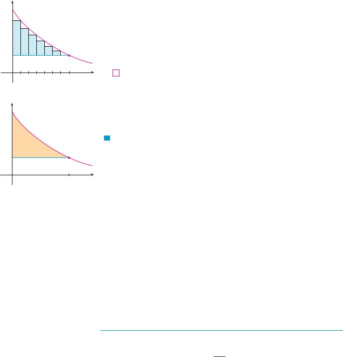
(This sum corresponds to the area enclosed by the rectangles in Figure 2.) If we let n l ,

P


this Riemann sum approaches the integral


X

0

xi

X

x

1

y0 p x P dx

FIGURE 2


which economists call the consumer surplus for the commodity.


The consumer surplus represents the amount of money saved by consumers in pur-

p


chasing the commodity at price P, corresponding to an amount demanded of X. Figure 3


p=p(x)


shows the interpretation of the consumer surplus as the area under the demand curve and


above the line p P.


consumer


V EXAMPLE 1 The demand for a product, in dollars, is


surplus

(X,P)


p 1200 0.2x 0.0001x 2

P

p=P


Find the consumer surplus when the sales level is 500.

0

X

x

SOLUTION Since the number of products sold is X 500, the corresponding price is

FIGURE 3


P 1200 0.2 500 0.0001 500 2 1075


Therefore, from Definition 1, the consumer surplus is


500

500


y0

p x P dx y0

1200 0.2x 0.0001x

2 1075 dx


500

125 0.2x 0.0001x 2

dx


y0


3


0


x 3

500


125x 0.1x 2 0.0001


0.0001 500 3


125 500 0.1 500 2


3


$33,333.33


M

BLOOD FLOW

In Example 7 in Section 3.7 we discussed the law of laminar flow:

v r P R2 r 2

4 l

which gives the velocity v of blood that flows along a blood vessel with radius R and length l at a distance r from the central axis, where P is the pressure difference between the ends of the vessel and is the viscosity of the blood. Now, in order to compute the rate of blood flow, or flux (volume per unit time), we consider smaller, equally spaced radii r1, r2, . . . .

552 |||| CHAPTER 8 FURTHER APPLICATIONS OF INTEGRATION

Îr

ri

FIGURE 4

FIGURE 5

The approximate area of the ring (or washer) with inner radius ri 1 and outer radius ri is

2 ri r

where r ri ri 1

(See Figure 4.) If r is small, then the velocity is almost constant throughout this ring and can be approximated by v ri . Thus the volume of blood per unit time that flows across the ring is approximately

2 ri r v ri 2 ri v ri r

and the total volume of blood that flows across a cross-section per unit time is approxi-

mately

n

2 ri v ri r

i 1

This approximation is illustrated in Figure 5. Notice that the velocity (and hence the volume per unit time) increases toward the center of the blood vessel. The approximation gets better as n increases. When we take the limit we get the exact value of the flux (or discharge), which is the volume of blood that passes a cross-section per unit time:


n


R 2 r v r dr


F lim


2 ri v ri r


n l i 1


y0


R


P


y0 2 r


R2 r 2 dr


4 l


P


P


r 2

r 4

r R


R


R2


y0


R2r r 3 dr


2 l


2 l

2

4


r 0


P


R4

R4


PR4


2 l


2

4


8 l


The resulting equation


2


F


PR4


8 l


aorta

vein

pulmonary


arteries

pulmonary

pulmonary

arteries

veins

right

left

atrium

atrium

pulmonary


veins


vein

FIGURE 6

is called Poiseuille’s Law; it shows that the flux is proportional to the fourth power of the radius of the blood vessel.

CARDIAC OUTPUT

Figure 6 shows the human cardiovascular system. Blood returns from the body through the veins, enters the right atrium of the heart, and is pumped to the lungs through the pulmonary arteries for oxygenation. It then flows back into the left atrium through the pulmonary veins and then out to the rest of the body through the aorta. The cardiac output of the heart is the volume of blood pumped by the heart per unit time, that is, the rate of flow into the aorta.

The dye dilution method is used to measure the cardiac output. Dye is injected into the right atrium and flows through the heart into the aorta. A probe inserted into the aorta measures the concentration of the dye leaving the heart at equally spaced times over a time interval 0, T until the dye has cleared. Let c t be the concentration of the dye at time t. If we divide 0, T into subintervals of equal length t, then the amount of dye that flows past the measuring point during the subinterval from t ti 1 to t ti is approximately

concentration volume c ti F t

SECTION 8.4 APPLICATIONS TO ECONOMICS AND BIOLOGY |||| 553

where F is the rate of flow that we are trying to determine. Thus the total amount of dye is approximately

n

n

c ti F t F c ti t

i 1

i 1

and, letting n l , we find that the amount of dye is

A F yT c t dt

0

Thus the cardiac output is given by

t

c t

t

c t


0

0

6

6.1

1

0.4

7

4.0

2

2.8

8

2.3

3

6.5

9

1.1

4

9.8

10

0

5

8.9


3

F

A


yT c t dt

0

where the amount of dye A is known and the integral can be approximated from the concentration readings.

V EXAMPLE 2 A 5-mg bolus of dye is injected into a right atrium. The concentration of the dye (in milligrams per liter) is measured in the aorta at one-second intervals as shown in the chart. Estimate the cardiac output.

SOLUTION Here A 5, t 1, and T 10. We use Simpson’s Rule to approximate the integral of the concentration:

10


y0 c t dt 31

0

4 0.4 2 2.8 4 6.5 2 9.8 4 8.9

2 6.1 4 4.0 2 2.3 4 1.1 0

41.87

Thus Formula 3 gives the cardiac output to be

F


A


5

0.12 L s 7.2 L min

10


41.87


y0

c t dt


8.4EXERCISES

M

1.The marginal cost function C x was defined to be the derivative of the cost function. (See Sections 3.7 and 4.7.)

If the marginal cost of maufacturing x meters of a fabric is C x 5 0.008x 0.000009x 2 (measured in dollars per meter) and the fixed start-up cost is C 0 $20,000, use the Net Change Theorem to find the cost of producing the first 2000 units.

2.The marginal revenue from the sale of x units of a product is 12 0.0004 x. If the revenue from the sale of the first 1000 units is $12,400, find the revenue from the sale of the first 5000 units.

3.The marginal cost of producing x units of a certain product is 74 1.1x 0.002x 2 0.00004x 3 (in dollars per unit). Find the increase in cost if the production level is raised from 1200 units to 1600 units.

4.The demand function for a certain commodity is p 20 0.05x. Find the consumer surplus when the sales level is 300. Illustrate by drawing the demand curve and identifying the consumer surplus as an area.

5.A demand curve is given by p 450 x 8 . Find the consumer surplus when the selling price is $10.

6.The supply function pS x for a commodity gives the relation between the selling price and the number of units that manufacturers will produce at that price. For a higher price, manufacturers will produce more units, so pS is an increasing

function of x. Let X be the amount of the commodity currently produced and let P pS X be the current price. Some producers would be willing to make and sell the commodity for a lower selling price and are therefore receiving more than their minimal price. The excess is called the producer surplus. An

554 |||| CHAPTER 8 FURTHER APPLICATIONS OF INTEGRATION

argument similar to that for consumer surplus shows that the surplus is given by the integral

yX P pS x dx

0

Calculate the producer surplus for the supply function

pS x 3 0.01x 2 at the sales level X 10. Illustrate by drawing the supply curve and identifying the producer surplus as an area.

7.If a supply curve is modeled by the equation

p 200 0.2x 3 / 2, find the producer surplus when the selling price is $400.

8.For a given commodity and pure competition, the number of units produced and the price per unit are determined as the

coordinates of the point of intersection of the supply and

demand curves. Given the demand curve p 50 201 x and the supply curve p 20 101 x, find the consumer surplus and the producer surplus. Illustrate by sketching the supply and demand curves and identifying the surpluses as areas.

;9. A company modeled the demand curve for its product

(in dollars) by the equation

p

800,000e x 5000

x 20,000

Use a graph to estimate the sales level when the selling price is $16. Then find (approximately) the consumer surplus for this sales level.

10.A movie theater has been charging $7.50 per person and selling about 400 tickets on a typical weeknight. After surveying their customers, the theater estimates that for every 50 cents that they lower the price, the number of moviegoers will increase by 35 per night. Find the demand function and calculate the consumer surplus when the tickets are priced at $6.00.

11.If the amount of capital that a company has at time t is f t , then the derivative, f t , is called the net investment flow. Suppose that the net investment flow is st million dollars per year (where t is measured in years). Find the increase in capital (the capital formation) from the fourth year to the eighth year.

12.If revenue flows into a company at a rate of

f t 9000s1 2t , where t is measured in years and f t is measured in dollars per year, find the total revenue obtained in the first four years.

13.Pareto’s Law of Income states that the number of people with

incomes between x a and x b is N xab Ax k dx, where A and k are constants with A 0 and k 1. The average income of these people is

x1 yb Ax 1 k dx N a

Calculate x.

14.A hot, wet summer is causing a mosquito population explosion in a lake resort area. The number of mosquitos is increasing at an estimated rate of 2200 10e0.8t per week (where t is measured in weeks). By how much does the mosquito population increase between the fifth and ninth weeks of summer?

15.Use Poiseuille’s Law to calculate the rate of flow in a small

human artery where we can take 0.027, R 0.008 cm, l 2 cm, and P 4000 dynes cm2.

16. High blood pressure results from constriction of the arteries. To maintain a normal flow rate (flux), the heart has to pump harder, thus increasing the blood pressure. Use Poiseuille’s Law to show that if R0 and P0 are normal values of the radius and pressure in an artery and the constricted values are R and P, then for the flux to remain constant, P and R are related by the equation

P R0 4 P0 R

Deduce that if the radius of an artery is reduced to threefourths of its former value, then the pressure is more than tripled.

17.The dye dilution method is used to measure cardiac output with 6 mg of dye. The dye concentrations, in mg L, are modeled by c t 20te 0.6t, 0 t 10, where t is measured in seconds. Find the cardiac output.

18.After an 8-mg injection of dye, the readings of dye concentration, in mg L, at two-second intervals are as shown in the table. Use Simpson’s Rule to estimate the cardiac output.

t

c t

t

c t


0

0

12

3.9

2

2.4

14

2.3

4

5.1

16

1.6

6

7.8

18

0.7

8

7.6

20

0

10

5.4


19.The graph of the concentration function c t is shown after a 7-mg injection of dye into a heart. Use Simpson’s Rule to estimate the cardiac output.

y

(mg/L)

6

4

2

0

2

4

6

8

10

12 14 t (seconds)

Соседние файлы в предмете [НЕСОРТИРОВАННОЕ]