SECTION 1.6 INVERSE FUNCTIONS AND LOGARITHMS |||| 59
25.Under ideal conditions a certain bacteria population is known to double every three hours. Suppose that there are initially 100 bacteria.
(a)What is the size of the population after 15 hours?
(b)What is the size of the population after t hours?
(c)Estimate the size of the population after 20 hours.
;(d) Graph the population function and estimate the time for the population to reach 50,000.
26.A bacterial culture starts with 500 bacteria and doubles in size every half hour.
(a)How many bacteria are there after 3 hours?
(b)How many bacteria are there after t hours?
(c)How many bacteria are there after 40 minutes?
;(d) Graph the population function and estimate the time for the population to reach 100,000.
;27. Use a graphing calculator with exponential regression capability to model the population of the world with the data from 1950 to 2000 in Table 1 on page 55. Use the model to estimate the population in 1993 and to predict the population in the year 2010.
;28. The table gives the population of the United States, in millions, for the years 1900–2000. Use a graphing calculator with exponential regression capability to model the US
population since 1900. Use the model to estimate the population in 1925 and to predict the population in the years 2010 and 2020.
Year |
Population |
Year |
Population |
|
|
|
|
1900 |
76 |
1960 |
179 |
1910 |
92 |
1970 |
203 |
1920 |
106 |
1980 |
227 |
1930 |
123 |
1990 |
250 |
1940 |
131 |
2000 |
281 |
1950 |
150 |
|
|
|
|
|
|
;29. If you graph the function
1 ! e1&x f #x$ ! 1 " e1&x
you’ll see that f appears to be an odd function. Prove it. ;30. Graph several members of the family of functions
1
f #x$ ! 1 " aebx
where a & 0. How does the graph change when b changes? How does it change when a changes?
 1.6 INVERSE FUNCTIONS AND LOGARITHMS
Table 1 gives data from an experiment in which a bacteria culture started with 100 bacteria in a limited nutrient medium; the size of the bacteria population was recorded at hourly intervals. The number of bacteria N is a function of the time t: N ! f #t$.
Suppose, however, that the biologist changes her point of view and becomes interested in the time required for the population to reach various levels. In other words, she is thinking of t as a function of N. This function is called the inverse function of f, denoted by f !1, and read “f inverse.” Thus t ! f !1#N$ is the time required for the population level to reach N. The values of f !1 can be found by reading Table 1 from right to left or by consulting Table 2. For instance, f !1#550$ ! 6 because f #6$ ! 550.
TABLE 1 |
N as a function of t |
|
|
|
t |
|
N ! f #t$ |
(hours) |
|
! population at time t |
|
|
|
0 |
|
100 |
1 |
|
168 |
2 |
|
259 |
3 |
|
358 |
4 |
|
445 |
5 |
|
509 |
6 |
|
550 |
7 |
|
573 |
8 |
|
586 |
|
|
|
TABLE 2 t as a function of N
|
t ! f !1#N$ |
N |
! time to reach N bacteria |
|
|
100 |
0 |
168 |
1 |
259 |
2 |
358 |
3 |
445 |
4 |
509 |
5 |
550 |
6 |
573 |
7 |
586 |
8 |
|
|
60 |||| CHAPTER 1 FUNCTIONS AND MODELS
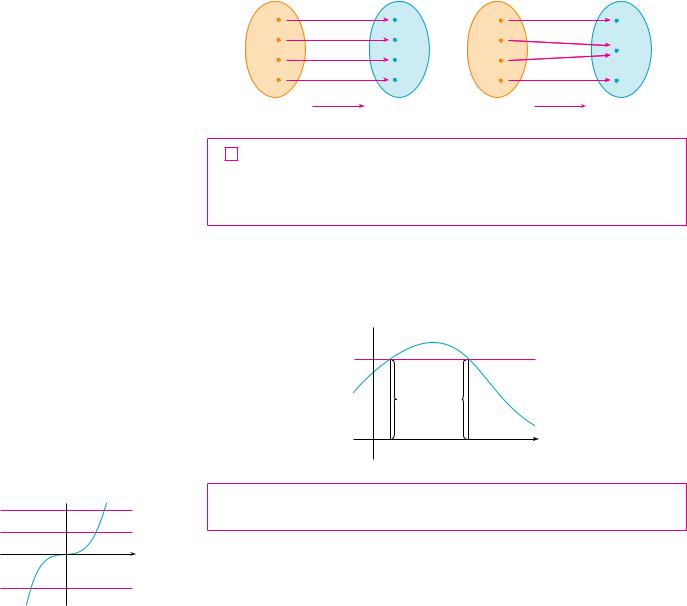
Not all functions possess inverses. Let’s compare the functions f and t whose arrow diagrams are shown in Figure 1. Note that f never takes on the same value twice (any two inputs in A have different outputs), whereas t does take on the same value twice (both 2 and 3 have the same output, 4). In symbols,
|
|
|
|
t!2" ! t!3" |
|
|
|
|
but |
|
f !x1 " " f !x2 " |
whenever x1 " x2 |
|
|
|
|
Functions that share this property with f are called one-to-one functions. |
|
|
|
4 |
|
10 |
4 |
|
10 |
|
|
3 |
|
7 |
3 |
|
4 |
|
|
2 |
|
4 |
2 |
|
|
|
|
|
|
|
FIGURE 1 |
1 |
f |
2 |
1 |
g |
2 |
|
A |
B |
|
|
|
f is one-to-one; g is not |
A |
B |
|
|
|
N In the language of inputs and outputs, this definition says that f is one-to-one if each output corresponds to only one input.
FIGURE 2
This function is not one-to-one because f(Ú)=f(Û).
1 DEFINITION A function f is called a one-to-one function if it never takes on
the same value twice; that is,
f !x1 " " f !x2 " whenever x1 " x2
If a horizontal line intersects the graph of f in more than one point, then we see from Figure 2 that there are numbers x1 and x2 such that f !x1 " ! f !x2 ". This means that f is not one-to-one. Therefore we have the following geometric method for determining whether a function is one-to-one.
y
y=Ä
ßà
y
y=þ
0x
FIGURE 3
Ä=þ is one-to-one.
HORIZONTAL LINE TEST A function is one-to-one if and only if no horizontal line intersects its graph more than once.
|
|
|
|
|
|
EXAMPLE 1 Is the function f !x" ! x3 one-to-one? |
|
V |
|
SOLUTION |
1 |
If x1 " x2 , then x13 " x23 (two different numbers can’t have the same cube). |
|
Therefore, by Definition 1, f !x" ! x3 is one-to-one. |
|
SOLUTION |
2 |
From Figure 3 we see that no horizontal line intersects the graph of f !x" ! x3 |
more than once. Therefore, by the Horizontal Line Test, f is one-to-one. |
M |
62 |||| CHAPTER 1 FUNCTIONS AND MODELS
|
The diagram in Figure 6 makes it clear how f !1 reverses the effect of f |
in this case. |
|
A |
B |
A |
B |
|
1 |
5 |
1 |
5 |
|
3 |
7 |
3 |
7 |
FIGURE 6 |
8 |
_10 |
8 |
_10 |
|
|
|
|
The inverse function reverses |
|
f |
f Ð! |
M |
inputs and outputs. |
|
|
|
The letter x is traditionally used as the independent variable, so when we concentrate on f !1 rather than on f, we usually reverse the roles of x and y in Definition 2 and write
3 |
f !1!x" ! y &? f ! y" ! x |
|
|
By substituting for y in Definition 2 and substituting for x in (3), we get the following cancellation equations:
4 |
f !1! f !x"" ! x |
for every x in A |
|
f ! f !1!x"" ! x |
for every x in B |
|
|
|
The first cancellation equation says that if we start with x, apply f, and then apply f !1, we arrive back at x, where we started (see the machine diagram in Figure 7). Thus f !1 undoes what f does. The second equation says that f undoes what f !1 does.
x  f
f  Ä
Ä  f Ð!
f Ð!  x
x
FIGURE 7
For example, if f !x" ! x3, then f !1!x" ! x1% 3 and so the cancellation equations become f !1! f !x"" ! !x3 "1% 3 ! x
f ! f !1!x"" ! !x1% 3 "3 ! x
These equations simply say that the cube function and the cube root function cancel each other when applied in succession.
Now let’s see how to compute inverse functions. If we have a function y ! f !x" and are able to solve this equation for x in terms of y, then according to Definition 2 we must have x ! f !1! y". If we want to call the independent variable x, we then interchange x and y and arrive at the equation y ! f !1!x".
5 HOW TO FIND THE INVERSE FUNCTION OF A ONE-TO-ONE FUNCTION f
STEP 1 Write y ! f !x".
STEP 2 Solve this equation for x in terms of y (if possible).
STEP 3 To express f !1 as a function of x, interchange x and y.
The resulting equation is y ! f !1!x".
64 |||| CHAPTER 1 FUNCTIONS AND MODELS
then we have
Thus, if x " 0, then loga x is the exponent to which the base a must be raised to give x. For example, log10 0.001 ! !3 because 10!3 ! 0.001.
The cancellation equations (4), when applied to the functions f !x" ! ax and f !1!x" ! loga x, become
y |
y=x |
|
y=a¨,""a>1 |
|
0 |
x |
|
y=loga x, "a>1 |
FIGURE 11
7 |
loga!ax " ! x |
for every x ! ! |
|
aloga x ! x |
for every x " 0 |
The logarithmic function loga has domain !0, %" and range !. Its graph is the reflection of the graph of y ! ax about the line y ! x.
Figure 11 shows the case where a " 1. (The most important logarithmic functions have base a " 1.) The fact that y ! ax is a very rapidly increasing function for x " 0 is reflected in the fact that y ! loga x is a very slowly increasing function for x " 1.
Figure 12 shows the graphs of y ! loga x with various values of the base a " 1. Since loga 1 ! 0, the graphs of all logarithmic functions pass through the point !1, 0".
The following properties of logarithmic functions follow from the corresponding properties of exponential functions given in Section 1.5.
y |
|
|
|
|
y=logª"x |
|
|
|
|
|
|
|
|
|
|
|
|
|
|
|
|
1 |
|
|
y=log£"x |
|
|
|
|
|
|
|
|
|
|
|
|
|
|
|
|
|
|
|
|
|
|
|
|
|
|
|
0 |
|
1 |
y=log∞"x |
x |
|
|
|
|
|
|
y=logÁü"x |
|
|
|
|
|
|
|
|
|
|
|
|
|
|
|
|
FIGURE 12
N NOTATION FOR LOGARITHMS
Most textbooks in calculus and the sciences, as well as calculators, use the notation ln x for the natural logarithm and log x for the “common logarithm,” log10 x. In the more advanced mathematical and scientific literature and in computer languages, however, the notation log x usually denotes the natural logarithm.
LAWS OF LOGARITHMS If x and y are positive numbers, then 1. loga!xy" ! loga x $ loga y
2. loga&xy ' ! loga x ! loga y
3. loga!xr " ! r loga x (where r is any real number)
EXAMPLE 6 Use the laws of logarithms to evaluate log2 80 ! log2 5. |
|
SOLUTION Using Law 2, we have |
|
log2 80 ! log2 5 ! log2& |
80 |
' ! log2 16 ! 4 |
|
5 |
|
because 24 ! 16. |
M |
N AT U R A L L O G A R I T H M S
Of all possible bases a for logarithms, we will see in Chapter 3 that the most convenient choice of a base is the number e, which was defined in Section 1.5. The logarithm with base e is called the natural logarithm and has a special notation:
loge x ! ln x
SECTION 1.6 INVERSE FUNCTIONS AND LOGARITHMS |||| 65
If we put a ! e and replace loge with “ln” in (6) and (7), then the defining properties of the natural logarithm function become
ln x ! y &? |
ey ! x |
|
|
|
|
ln!ex " ! x |
x ! ! |
eln x ! x |
x " 0 |
|
|
In particular, if we set x ! 1, we get
ln e ! 1
EXAMPLE 7 Find x if ln x ! 5.
SOLUTION 1 From (8) we see that
ln x ! 5 means e5 ! x
Therefore x ! e5.
(If you have trouble working with the “ln” notation, just replace it by loge . Then the equation becomes loge x ! 5; so, by the definition of logarithm, e5 ! x.)
SOLUTION 2 Start with the equation
ln x ! 5
and apply the exponential function to both sides of the equation:
eln x ! e5 |
|
But the second cancellation equation in (9) says that eln x ! x. Therefore, x ! e5. |
M |
EXAMPLE 8 Solve the equation e5!3x ! 10. |
|
SOLUTION We take natural logarithms of both sides of the equation and use (9): |
|
ln!e5!3x " ! ln 10 |
|
5 ! 3x ! ln 10 |
|
3x ! 5 ! ln 10 |
|
x ! 31 !5 ! ln 10" |
|
Since the natural logarithm is found on scientific calculators, we can approximate the |
|
solution: to four decimal places, x ( 0.8991. |
M |
66 |||| CHAPTER 1 FUNCTIONS AND MODELS |
|
|
|
EXAMPLE 9 Express ln a $ 21 ln b as a single logarithm. |
|
|
V |
|
|
|
|
|
SOLUTION Using Laws 3 and 1 of logarithms, we have |
|
|
|
ln a $ 21 ln b ! ln a $ ln b1% 2 |
|
|
|
! ln a $ ln s |
|
|
|
b |
|
|
|
! ln(as |
|
) |
|
|
|
b |
M |
The following formula shows that logarithms with any base can be expressed in terms of the natural logarithm.
10 CHANGE OF BASE FORMULA For any positive number a !a " 1", we have
ln x loga x ! ln a
PROOF Let y ! loga x. Then, from (6), we have ay ! x. Taking natural logarithms of both sides of this equation, we get y ln a ! ln x. Therefore
Scientific calculators have a key for natural logarithms, so Formula 10 enables us to use a calculator to compute a logarithm with any base (as shown in the following example). Similarly, Formula 10 allows us to graph any logarithmic function on a graphing calculator or computer (see Exercises 41 and 42).
EXAMPLE 10 Evaluate log8 5 correct to six decimal places.
SOLUTION Formula 10 gives
log8 5 |
ln 5 |
( 0.773976 |
|
! ln 8 |
M |
The graphs of the exponential function y ! ex and its inverse function, the natural logarithm function, are shown in Figure 13. Because the curve y ! ex crosses the y-axis with a slope of 1, it follows that the reflected curve y ! ln x crosses the x-axis with a slope of 1.
In common with all other logarithmic functions with base greater than 1, the natural logarithm is an increasing function defined on !0, %" and the y-axis is a vertical asymptote. (This means that the values of ln x become very large negative as x approaches 0.)
EXAMPLE 11 Sketch the graph of the function y ! ln!x ! 2" ! 1.
SOLUTION We start with the graph of y ! ln x as given in Figure 13. Using the transformations of Section 1.3, we shift it 2 units to the right to get the graph of y ! ln!x ! 2" and then we shift it 1 unit downward to get the graph of y ! ln!x ! 2" ! 1. (See Figure 14.)

y
y=ln"x
FIGURE 14
y
FIGURE 15
y
y=Ïãx
20
y=ln"x
FIGURE 16
|
|
|
|
|
SECTION 1.6 |
INVERSE FUNCTIONS AND LOGARITHMS |
|||| 67 |
y |
|
x=2 |
|
|
|
y |
x=2 |
|
|
|
|
|
|
|
|
|
|
|
|
|
|
|
y=ln(x-2) |
|
|
y=ln(x-2)-1 |
|
|
|
|
|
|
|
|
|
|
|
|
0 |
2 |
|
|
(3,"0) |
x |
|
0 |
2 |
x |
 (3,"_1)
M
Although ln x is an increasing function, it grows very slowly when x " 1. In fact, ln x grows more slowly than any positive power of x. To illustrate this fact, we compare approximate values of the functions y ! ln x and y ! x1% 2 ! sx in the following table and we graph them in Figures 15 and 16. You can see that initially the graphs of y ! sx and y ! ln x grow at comparable rates, but eventually the root function far surpasses the logarithm.
|
x |
|
1 |
2 |
5 |
10 |
50 |
100 |
500 |
1000 |
10,000 |
100,000 |
|
|
|
|
|
|
|
|
|
|
|
|
|
|
|
|
ln x |
|
0 |
0.69 |
1.61 |
2.30 |
3.91 |
4.6 |
6.2 |
6.9 |
9.2 |
11.5 |
|
|
|
|
|
|
|
|
|
|
|
|
|
|
|
|
s |
|
|
|
1 |
1.41 |
2.24 |
3.16 |
7.07 |
10.0 |
22.4 |
31.6 |
100 |
316 |
|
x |
|
|
ln x |
|
0 |
0.49 |
0.72 |
0.73 |
0.55 |
0.46 |
0.28 |
0.22 |
0.09 |
0.04 |
|
|
|
|
|
|
sx |
|
|
|
|
|
|
|
|
|
|
|
|
|
|
|
|
|
|
|
|
|
|
|
|
|
|
|
I N V E R S E T R I G O N O M E T R I C F U N C T I O N S
When we try to find the inverse trigonometric functions, we have a slight difficulty: Because the trigonometric functions are not one-to-one, they don’t have inverse functions. The difficulty is overcome by restricting the domains of these functions so that they become one-to-one.
You can see from Figure 17 that the sine function y ! sin x is not one-to-one (use the Horizontal Line Test). But the function f !x" ! sin x, !&%2 ' x ' &%2, is one-to-one (see Figure 18). The inverse function of this restricted sine function f exists and is denoted by sin!1 or arcsin. It is called the inverse sine function or the arcsine function.
|
|
|
y |
|
|
y=sin"x |
|
_π2 |
y |
|
|
|
|
|
|
|
|
|
|
|
|
|
|
|
|
|
|
|
|
|
|
|
|
|
|
|
|
|
|
|
|
|
|
|
|
|
|
|
|
|
|
|
|
|
|
|
|
|
|
|
|
|
|
|
|
|
|
|
|
_ |
|
π |
|
|
0 π |
π |
x |
|
|
0 π |
x |
|
|
|
|
|
2 |
|
|
|
|
|
|
|
|
|
2 |
|
|
|
|
|
|
|
|
|
|
|
|
|
|
FIGURE 17 |
|
|
|
|
|
|
|
|
FIGURE 18 |
y=sin"x, _π2 øxøπ2 |
Since the definition of an inverse function says that
f !1!x" ! y &? f ! y" ! x
68 |||| CHAPTER 1 FUNCTIONS AND MODELS
| sin!1x " sin1 x
3
1
¬ 2"Ïã2
we have
sin!1x ! y &? |
sin y ! x and |
! |
& |
' y ' |
& |
|
|
|
|
2 |
2 |
|
|
|
|
|
|
|
|
Thus, if !1 ' x ' 1, sin!1x is the number between !&%2 and &%2 whose sine is x.
EXAMPLE 12 Evaluate (a) sin!1(12) and (b) tan(arcsin 13 ).
SOLUTION |
|
|
(a) We have |
sin!1(21) ! |
& |
|
|
|
|
6 |
|
|
because sin!&%6" ! 12 and &%6 lies between !&%2 and &%2.
(b) Let ( ! arcsin 13 , so sin ( ! 13. Then we can draw a right triangle with angle ( as in Figure 19 and deduce from the Pythagorean Theorem that the third side has length
s9 ! 1 ! 2s2 . This enables us to read from the triangle that
|
tan(arcsin 31 ) ! tan ( ! |
1 |
|
|
|
|
|
|
M |
|
|
2s |
|
|
|
|
|
|
|
2 |
|
|
|
|
The cancellation equations for inverse functions become, in this case, |
|
|
|
|
|
|
|
|
|
|
|
|
|
|
|
sin!1!sin x" ! x for ! |
& |
|
' x ' |
& |
|
|
|
|
|
|
|
|
|
|
2 |
|
2 |
|
|
|
|
|
|
|
|
|
|
|
|
|
|
|
sin!sin!1x" ! x for !1 ' x ' 1 |
|
|
|
|
|
|
|
|
The inverse sine function, sin!1, has domain #!1, 1$ and range #!&%2, |
&%2$, and its |
graph, shown in Figure 20, is obtained from that of the restricted sine function (Figure 18) by reflection about the line y ! x.
|
|
|
y |
|
|
|
|
|
|
|
|
y |
|
|
|
|
|
|
|
|
|
|
|
|
|
|
|
|
|
|
|
|
|
|
|
|
|
|
|
|
|
|
|
π |
|
|
|
|
|
|
|
|
|
|
|
|
|
|
|
|
|
|
|
|
2 |
|
|
|
|
|
|
|
|
1 |
|
|
|
|
|
|
|
|
|
|
|
|
|
|
|
|
|
|
|
|
|
|
|
|
|
|
|
|
|
|
|
|
|
|
|
|
|
|
|
|
|
|
|
|
|
|
|
|
|
|
|
|
|
|
|
|
|
|
|
|
|
|
|
|
|
|
|
|
|
|
|
|
|
|
|
|
|
|
|
|
|
|
_ |
|
1 |
|
0 |
1 |
x |
|
0 |
|
|
|
π |
π |
x |
|
|
|
|
|
|
|
|
|
|
|
|
|
|
|
|
|
2 |
|
|
|
|
|
|
|
|
|
|
|
_π2 |
|
|
|
|
|
|
|
|
|
|
|
|
|
|
|
|
|
|
|
FIGURE 20 |
|
|
|
|
|
|
|
|
|
|
|
|
|
|
|
|
|
|
|
|
|
|
|
|
|
|
|
FIGURE 21 |
|
|
|
|
|
|
|
|
|
y=sinÐ! x=arcsin x |
|
|
y=cos"x, 0øxøπ |
|
|
|
|
|
|
The inverse |
cosine |
function is |
handled similarly. The restricted cosine function |
|
f !x" ! cos x, 0 ' x ' |
&, is one-to-one (see Figure 21) and so it has an inverse function |
denoted by cos!1 or arccos. |
|
|
|
|
|
|
|
|
|
|
|
|
|
cos!1x ! y &? cos y ! x and

y
π
π
2
FIGURE 22
y=cosÐ!"x=arccos x
y
FIGURE 23 y=tan"x, _π2 <x<π2
Пггггг1+≈
y
1
FIGURE 24
|
|
|
SECTION 1.6 INVERSE FUNCTIONS AND LOGARITHMS |
|||| 69 |
|
The cancellation equations are |
|
|
|
|
|
|
|
|
|
|
|
|
|
|
|
|
|
|
cos!1!cos x" ! x |
for 0 ' x ' & |
|
|
|
|
|
|
|
|
|
|
cos!cos!1x" ! x for !1 ' x ' 1 |
|
|
|
|
|
|
|
|
The inverse cosine function, cos!1, has domain #!1, 1$ and range #0, |
&$. Its graph is |
x |
shown in Figure 22. |
|
|
|
|
|
|
|
|
|
|
|
|
|
|
|
|
The |
tangent function can |
be |
made one-to-one by restricting |
it |
to the |
interval |
|
!!&%2, |
&%2". Thus the inverse tangent function is defined as the inverse of the function |
|
f !x" ! tan x, !&%2 * x * &%2. (See Figure 23.) It is denoted by tan!1 or arctan. |
|
|
|
|
|
|
|
|
|
|
|
|
|
|
|
|
|
|
|
|
|
|
|
|
tan!1x ! y |
&? tan y ! x and ! |
& |
|
* y * |
& |
|
|
|
|
|
|
2 |
|
2 |
|
|
|
|
|
|
|
|
|
|
|
|
|
|
|
|
|
|
|
|
|
|
|
|
|
|
|
|
|
|
|
|
|
|
|
EXAMPLE 13 Simplify the expression cos!tan!1x". |
|
|
|
|
|
|
|
|
|
|
SOLUTION |
1 Let y ! tan!1x. Then tan y ! x and !&%2 * y * &%2. We want to find cos y |
|
but, since tan y is known, it is easier to find sec y first: |
|
|
|
|
|
|
|
|
|
|
|
|
sec2 y ! 1 $ tan2 y ! 1 $ x2 |
|
|
|
|
|
|
|
|
|
|
|
|
sec y ! s |
|
|
|
|
|
|
|
|
1 $ x2 |
!since sec y " 0 for !&%2 * y * &%2" |
|
|
|
Thus |
|
cos!tan!1x" |
! cos y |
1 |
|
|
|
1 |
|
|
|
|
|
|
|
|
|
|
! |
|
! |
|
|
|
|
|
|
|
|
|
|
|
sec y |
s |
|
|
|
|
|
|
|
|
1 |
$ x2 |
|
|
|
|
|
xSOLUTION 2 Instead of using trigonometric identities as in Solution 1, it is perhaps easier to use a diagram. If y ! tan!1x, then tan y ! x, and we can read from Figure 24 (which
illustrates the case y " 0) that
cos!tan!1x" ! cos y ! 1 s1 $ x2
The inverse tangent function, tan!1 ! arctan, has domain ! and range Its graph is shown in Figure 25.
FIGURE 25 y=tanÐ!"x=arctan"x
We know that the lines x ! )&%2 are vertical asymptotes of the graph of tan. Since the graph of tan!1 is obtained by reflecting the graph of the restricted tangent function about the line y ! x, it follows that the lines y ! &%2 and y ! !&%2 are horizontal asymptotes of the graph of tan!1.
70 |||| CHAPTER 1 FUNCTIONS AND MODELS
The remaining inverse trigonometric functions are not used as frequently and are sum-
|
|
|
|
|
|
|
|
|
|
|
|
|
|
|
|
|
|
marized here. |
|
|
|
|
|
|
|
|
|
|
|
|
|
|
|
|
|
|
|
|
|
|
|
|
|
|
|
|
|
|
|
|
|
|
|
|
|
|
|
|
|
|
|
|
|
|
|
|
|
|
|
|
|
|
|
|
|
y ! csc |
!1 |
x |
$& x & # 1# |
&? |
csc y ! x |
and |
y ! $0, |
"2% " $ , 3 "2% |
|
|
y |
|
|
|
|
|
|
|
|
|
|
|
|
|
|
11 |
|
|
|
|
|
|
|
" |
" |
" |
|
|
|
|
|
|
|
|
|
|
|
|
|
|
|
|
|
y ! sec!1x |
$& x & # 1# |
&? |
sec y ! x |
and |
y ! !0, |
""2# " !", 3""2# |
|
|
|
|
|
|
|
|
|
|
|
|
|
|
|
|
|
|
|
|
|
|
|
|
|
|
|
|
|
|
|
|
|
|
|
|
|
|
|
|
|
|
|
|
|
|
|
|
|
|
|
|
|
|
y ! cot!1x $x ! !# |
&? |
cot y ! x |
and |
y ! $0, |
"# |
|
|
_1 |
|
|
|
0 |
|
π |
|
2π |
|
x |
|
|
|
|
|
|
|
|
|
|
|
|
|
|
|
|
|
|
|
|
|
|
|
|
|
|
|
|
|
|
|
|
|
|
|
|
|
|
|
|
|
|
|
|
|
|
|
|
|
|
|
|
|
|
|
|
|
|
|
|
|
|
|
The choice of intervals for y in the definitions of csc!1 and sec!1 is not universally |
|
|
|
|
|
|
|
|
|
|
|
|
|
|
|
|
|
|
|
|
|
|
|
|
|
|
|
|
|
|
|
|
|
|
|
|
agreed upon. For instance, some authors use y ! !0, ""2# " $""2, |
"% in the definition of |
|
|
|
|
|
|
|
|
|
|
|
|
|
|
|
|
|
|
FIGURE 26 |
|
|
|
|
|
|
|
|
|
|
|
sec!1. [You can see from the graph of the secant function in Figure 26 that both this choice |
y=sec!x |
|
|
|
|
|
|
|
|
|
|
|
|
and the one in (11) will work.] |
|
|
|
|
|
|
|
1.6E X E R C I S E S
1.(a) What is a one-to-one function?
(b)How can you tell from the graph of a function whether it is one-to-one?
2.(a) Suppose f is a one-to-one function with domain A and range B. How is the inverse function f !1 defined? What is the domain of f !1? What is the range of f !1?
(b)If you are given a formula for f, how do you find a formula for f !1?
(c)If you are given the graph of f, how do you find the graph of f !1?
3–14 A function is given by a table of values, a graph, a formula, or a verbal description. Determine whether it is one-to-one.
3. |
|
|
|
|
|
|
|
|
|
|
|
|
|
|
x |
1 |
2 |
|
3 |
4 |
5 |
6 |
|
|
|
|
|
|
|
|
|
|
|
|
|
|
|
|
|
|
f $x# |
1.5 |
2.0 |
|
3.6 |
5.3 |
2.8 |
2.0 |
|
4. |
|
|
|
|
|
|
|
|
|
|
|
|
|
|
|
|
|
|
|
|
|
|
|
|
|
|
|
x |
1 |
2 |
|
3 |
4 |
5 |
6 |
|
|
|
|
|
|
|
|
|
|
|
|
|
|
|
|
|
|
f $x# |
1 |
2 |
|
4 |
8 |
16 |
32 |
|
|
|
|
|
|
|
|
|
|
|
|
|
|
|
5. |
|
|
y |
|
|
|
|
6. |
|
y |
|
|
|
|
|
|
|
|
|
|
|
|
|
|
|
|
|
|
|
|
|
|
|
|
|
|
|
|
|
|
|
|
|
|
|
x |
|
|
|
|
|
|
x |
|
|
|
|
|
|
|
|
|
|
|
|
|
|
|
|
|
|
7. |
y |
|
x |
9. |
f $x# ! x2 ! 2x |
11. |
t$x# ! 1"x |
8.y
x
10. f $x# ! 10 ! 3x 12. t$x# ! cos x
13.f $t# is the height of a football t seconds after kickoff.
14.f $t# is your height at age t.
15. |
If |
f is a one-to-one function such that f $2# ! 9, what |
|
is |
f !1$9#? |
|
|
16. |
Let f $x# ! 3 |
$ x2 |
$ tan$"x"2#, where !1 % x % 1. |
(a)Find f !1$3#.
(b)Find f $ f !1$5##.
17.If t$x# ! 3 $ x $ ex, find t!1$4#.
18.The graph of f is given.
(a)Why is f one-to-one?
(b)What are the domain and range of f !1?
(c)What is the value of f !1$2#?
(d)Estimate the value of f !1$0#.
y
1
0 1 x
19.The formula C ! 59 $F ! 32#, where F # !459.67, expresses the Celsius temperature C as a function of the Fahrenheit temperature F. Find a formula for the inverse function and interpret it. What is the domain of the inverse function?
20.In the theory of relativity, the mass of a particle with speed v is
m ! f $v# ! m0
s1 ! v 2"c2
where m0 is the rest mass of the particle and c is the speed of light in a vacuum. Find the inverse function of f and explain its meaning.


 (a,"b)


