

- •CONTENTS
- •Preface
- •To the Student
- •Diagnostic Tests
- •1.1 Four Ways to Represent a Function
- •1.2 Mathematical Models: A Catalog of Essential Functions
- •1.3 New Functions from Old Functions
- •1.4 Graphing Calculators and Computers
- •1.6 Inverse Functions and Logarithms
- •Review
- •2.1 The Tangent and Velocity Problems
- •2.2 The Limit of a Function
- •2.3 Calculating Limits Using the Limit Laws
- •2.4 The Precise Definition of a Limit
- •2.5 Continuity
- •2.6 Limits at Infinity; Horizontal Asymptotes
- •2.7 Derivatives and Rates of Change
- •Review
- •3.2 The Product and Quotient Rules
- •3.3 Derivatives of Trigonometric Functions
- •3.4 The Chain Rule
- •3.5 Implicit Differentiation
- •3.6 Derivatives of Logarithmic Functions
- •3.7 Rates of Change in the Natural and Social Sciences
- •3.8 Exponential Growth and Decay
- •3.9 Related Rates
- •3.10 Linear Approximations and Differentials
- •3.11 Hyperbolic Functions
- •Review
- •4.1 Maximum and Minimum Values
- •4.2 The Mean Value Theorem
- •4.3 How Derivatives Affect the Shape of a Graph
- •4.5 Summary of Curve Sketching
- •4.7 Optimization Problems
- •Review
- •5 INTEGRALS
- •5.1 Areas and Distances
- •5.2 The Definite Integral
- •5.3 The Fundamental Theorem of Calculus
- •5.4 Indefinite Integrals and the Net Change Theorem
- •5.5 The Substitution Rule
- •6.1 Areas between Curves
- •6.2 Volumes
- •6.3 Volumes by Cylindrical Shells
- •6.4 Work
- •6.5 Average Value of a Function
- •Review
- •7.1 Integration by Parts
- •7.2 Trigonometric Integrals
- •7.3 Trigonometric Substitution
- •7.4 Integration of Rational Functions by Partial Fractions
- •7.5 Strategy for Integration
- •7.6 Integration Using Tables and Computer Algebra Systems
- •7.7 Approximate Integration
- •7.8 Improper Integrals
- •Review
- •8.1 Arc Length
- •8.2 Area of a Surface of Revolution
- •8.3 Applications to Physics and Engineering
- •8.4 Applications to Economics and Biology
- •8.5 Probability
- •Review
- •9.1 Modeling with Differential Equations
- •9.2 Direction Fields and Euler’s Method
- •9.3 Separable Equations
- •9.4 Models for Population Growth
- •9.5 Linear Equations
- •9.6 Predator-Prey Systems
- •Review
- •10.1 Curves Defined by Parametric Equations
- •10.2 Calculus with Parametric Curves
- •10.3 Polar Coordinates
- •10.4 Areas and Lengths in Polar Coordinates
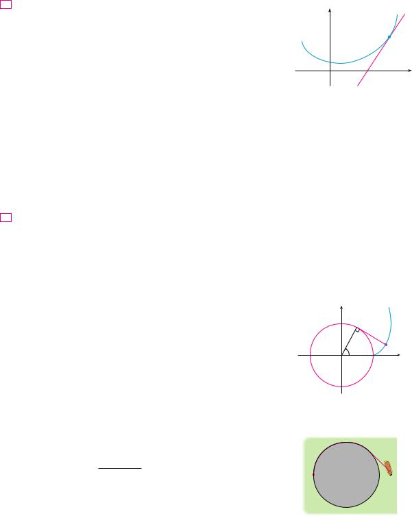
- •10.5 Conic Sections
- •10.6 Conic Sections in Polar Coordinates
- •Review
- •11.1 Sequences
- •11.2 Series
- •11.3 The Integral Test and Estimates of Sums
- •11.4 The Comparison Tests
- •11.5 Alternating Series
- •11.6 Absolute Convergence and the Ratio and Root Tests
- •11.7 Strategy for Testing Series
- •11.8 Power Series
- •11.9 Representations of Functions as Power Series
- •11.10 Taylor and Maclaurin Series
- •11.11 Applications of Taylor Polynomials
- •Review
- •APPENDIXES
- •A Numbers, Inequalities, and Absolute Values
- •B Coordinate Geometry and Lines
- •E Sigma Notation
- •F Proofs of Theorems
- •G The Logarithm Defined as an Integral
- •INDEX

630 |||| CHAPTER 10 PARAMETRIC EQUATIONS AND POLAR COORDINATES
3.Now try b 1 and a n d, a fraction where n and d have no common factor. First let n 1 and try to determine graphically the effect of the denominator d on the shape of the graph. Then let n vary while keeping d constant. What happens when n d 1?
4.What happens if b 1 and a is irrational? Experiment with an irrational number like
s2 or e 2. Take larger and larger values for and speculate on what would happen if we were to graph the hypocycloid for all real values of .
5.If the circle C rolls on the outside of the fixed circle, the curve traced out by P is called an epicycloid. Find parametric equations for the epicycloid.
6.Investigate the possible shapes for epicycloids. Use methods similar to Problems 2–4.
10.2CALCULUS WITH PARAMETRIC CURVES
Having seen how to represent curves by parametric equations, we now apply the methods of calculus to these parametric curves. In particular, we solve problems involving tangents, area, arc length, and surface area.
TANGENTS
In the preceding section we saw that some curves defined by parametric equations x f t and y t t can also be expressed, by eliminating the parameter, in the form y F x . (See Exercise 67 for general conditions under which this is possible.) If we substitute
x f t and y t t in the equation y F x , we get
t t F f t
and so, if t, F, and f are differentiable, the Chain Rule gives
|
t t F f t f t F x f t |
|||
If f t 0, we can solve for F x : |
||||
1 |
F x |
t t |
|
|
f t |
||||
|
|
|||
N If we think of a parametric curve as being traced out by a moving particle, then dy dt and dx dt are the vertical and horizontal velocities of the particle and Formula 2 says that the slope of the tangent is the ratio of these velocities.
Since the slope of the tangent to the curve y F x at x, F x is F x , Equation 1 enables us to find tangents to parametric curves without having to eliminate the parameter. Using Leibniz notation, we can rewrite Equation 1 in an easily remembered form:
|
|
|
|
|
dy |
|
|
|
|
|
|
|
|
|
|
|
|
|
|
2 |
|
dy |
|
dt |
|
if |
dx |
0 |
|
|
dx |
|
|
|
|||||
|
|
|
|
dx |
|
|
dt |
||
|
|
|
|
|
dt |
|
|
|
|
|
|
|
|
|
|
|
|
|
|
It can be seen from Equation 2 that the curve has a horizontal tangent when dy dt 0 (provided that dx dt 0) and it has a vertical tangent when dx dt 0 (provided that dy dt 0). This information is useful for sketching parametric curves.
SECTION 10.2 CALCULUS WITH PARAMETRIC CURVES |||| 631
|
|
|
|
d 2y |
|
| Note that |
d 2y |
|
dt 2 |
|
|
2 |
2 |
|
|||
|
dx |
|
|
d x |
|
|
|
|
|
dt 2 |
|
As we know from Chapter 4, it is also useful to consider d2 y dx2. This can be found by replacing y by dy dx in Equation 2:
|
|
|
|
|
|
|
d |
|
dy |
|
||
d2 y |
|
d |
dy |
|
dt |
dx |
||||||
dx2 |
dx |
dx |
|
|
|
dx |
|
|||||
|
|
|
|
|
|
|
|
|
dt |
|||
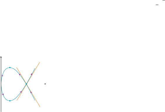
EXAMPLE 1 A curve C is defined by the parametric equations x t2, y t3 3t.
(a)Show that C has two tangents at the point (3, 0) and find their equations.
(b)Find the points on C where the tangent is horizontal or vertical.
(c)Determine where the curve is concave upward or downward.
(d)Sketch the curve.
SOLUTION
(a) Notice that y t3 3t t t2 3 0 when t 0 or t s3 . Therefore the point 3, 0 on C arises from two values of the parameter, t s3 and t s3 . This indicates that C crosses itself at 3, 0 . Since
|
dy |
|
|
|
dy dt |
|
|
|
3t2 3 |
|
3 |
1 |
|
|
|
||||||
|
|
|
|
|
|
|
|
|
|
t |
|
|
|||||||||
|
dx |
|
dx dt |
2t |
2 |
|
t |
||||||||||||||
the slope of the tangent when t s |
|
is dy dx |
|
6 (2s |
|
|
) s |
|
, so the equa- |
||||||||||||
3 |
|
3 |
3 |
||||||||||||||||||
tions of the tangents at 3, 0 are |
|
|
|
|
|
|
|
|
|
|
|
|
|
|
|
|
|||||
y s |
|
|
x 3 |
|
|
|
and |
y s |
|
x 3 |
|||||||||||
3 |
|
|
|
3 |
|||||||||||||||||
yy=œ„3(x-3) (b) C has a horizontal tangent when dy dx 0, that is, when dy dt 0 and dx dt 0.
t=_1 |
Since dy dt 3t2 3, this happens when t2 1, that is, t 1. The corresponding |
|
|
|
points on C are 1, 2 and (1, 2). C has a vertical tangent when dx dt 2t 0, that is, |
(1, 2) |
|
|
|
t 0. (Note that dy dt 0 there.) The corresponding point on C is (0, 0). |
|
|
|
|
(c) To determine concavity we calculate the second derivative:
|
|
|
(3, 0) |
|
|
|
|
|
|
|
|
|
|
|
|
|
|
|
|
|
1 |
|
|
|
|
|
|
|
|
||||||
0 |
|
|
x |
|
|
|
d |
dy |
3 |
1 |
|
|
|
|
|
||||||||||||||||||||
|
|
|
|
|
|
|
|
|
|
|
|
|
|
|
|||||||||||||||||||||
|
|
|
|
|
|
|
d2 y |
|
|
|
dt |
dx |
2 |
t2 |
3 t2 1 |
|
|
|
|||||||||||||||||
|
t=1 |
|
|
|
|
|
|
|
|
|
|
|
|
|
|
|
|
|
|
|
|
|
|
|
|
|
|
|
|
||||||
|
|
|
|
dx2 |
|
|
|
|
dx |
|
|
|
2t |
|
|
4t3 |
|
|
|
||||||||||||||||
(1,_2) |
|
|
|
|
|
|
|
|
|
|
|
|
|
|
|
|
|
|
|
|
|
|
|
|
|
|
|
|
|
|
|
|
|
||
|
|
|
|
|
|
|
|
|
|
|
|
|
dt |
|
|
|
|
|
|
|
|
|
|
|
|
|
|
|
|
||||||
|
|
|
|
|
|
|
|
|
|
|
|
|
|
|
|
|
|
|
|
|
|
|
|
|
|
|
|
|
|
|
|
||||
|
|
|
y=_œ3(x„-3) |
|
|
|
|
|
|
|
|
|
|
|
|
|
|
|
|
|
|
|
|
|
|
|
|
|
|
||||||
|
|
|
|
|
Thus the curve is concave upward when t 0 and concave downward when t 0. |
|
|||||||||||||||||||||||||||||
FIGURE 1 |
|
|
(d) Using the information from parts (b) and (c), we sketch C in Figure 1. |
M |
|||||||||||||||||||||||||||||||
|
|
|
|
|
|
EXAMPLE 2 |
|
|
|
|
|
|
|
|
|
|
|
|
|
|
|
|
|
|
|
|
|
|
|
|
|
|
|||
|
|
|
|
|
V |
|
|
|
|
|
|
|
|
|
|
|
|
|
|
|
|
|
|
|
|
|
|
|
|
|
|
||||
|
|
|
|
|
(a) Find the tangent to the cycloid x r sin , y r 1 cos |
at the point |
|
||||||||||||||||||||||||||||
|
|
|
|
|
where 3. (See Example 7 in Section 10.1.) |
|
|
|
|
|
|
|
|
||||||||||||||||||||||
|
|
|
|
|
(b) At what points is the tangent horizontal? When is it vertical? |
|
|
|
|||||||||||||||||||||||||||
|
|
|
|
|
SOLUTION |
|
|
|
|
|
|
|
|
|
|
|
|
|
|
|
|
|
|
|
|
|
|
|
|
|
|
||||
|
|
|
|
|
(a) The slope of the tangent line is |
|
|
|
|
|
|
|
|
|
|
|
|
|
|
|
|
||||||||||||||
|
|
|
|
|
|
|
|
dy |
|
|
dy d |
|
|
|
r sin |
|
|
sin |
|
|
|
||||||||||||||
|
|
|
|
|
|
|
|
dx |
|
dx d |
|
r 1 cos |
|
1 cos |
|
|
|
|
|||||||||||||||||
632 |||| CHAPTER 10 PARAMETRIC EQUATIONS AND POLAR COORDINATES
When
3, we have
3 |
|
|
sin |
x r |
3
r
3
s23
y r 1 cos
3
2r
and |
dy |
|
sin 3 |
|
s |
3 |
2 |
s |
|
|
|
|
3 |
||||||||
dx |
1 cos 3 |
|
|
1 |
||||||
|
|
1 2 |
|
|
||||||
Therefore the slope of the tangent is s3 and its equation is
|
|
|
|
|
|
|
|
|
|
|
|
|
|
|
|
|
|
|
|
|
y |
r |
|
|
|
|
x |
r |
|
rs3 |
|
|
or |
|
|
|
|
||||
|
3 |
|
|
|
|
3 |
x y r |
|||||||||||||
|
|
|
|
|
|
|
|
|
|
|
|
|||||||||
2 |
|
s |
|
|
3 |
2 |
|
|
|
s |
|
|
s3 |
|||||||
The tangent is sketched in Figure 2.
2
|
|
|
y |
|
|
(πr,2r) |
|
(3πr,2r) |
(5πr,2r) |
|||||
|
(_πr,2r) |
|
|
|
||||||||||
|
|
|
|
|
|
|
|
|
|
|
|
|
|
|
|
|
|
|
|
¨= |
π |
|
|
|
|
|
|
|
|
|
|
|
|
3 |
|
|
|
|
|
|
||||
FIGURE 2 |
|
0 |
|
|
|
2πr |
|
4πr |
|
x |
||||
|
|
|
|
|
|
|
|
|
|
|
||||
(b) The tangent is horizontal when dy dx 0, which occurs when sin 0 and |
||||||||||||||
1 cos 0, that is, |
2n 1 , n an integer. The corresponding point on the |
|||||||||||||
cycloid is 2n 1 r, 2r .
When 2n , both dx d and dy d are 0. It appears from the graph that there are vertical tangents at those points. We can verify this by using l’Hospital’s Rule as follows:
N The limits of integration for t are found as usual with the Substitution Rule. When x a, t is either or . When x b, t is the remaining value.
lim |
dy |
|
lim |
|
sin |
lim |
cos |
|
|
|
cos |
sin |
|||||
l2n dx |
|
l2n 1 |
l2n |
|
||||
A similar computation shows that dy dx l as l 2n , so indeed there are verti-
cal tangents when 2n , that is, when x 2n r. |
M |
AREAS
We know that the area under a curve y F x from a to b is A xab F x dx, where F x 0. If the curve is traced out once by the parametric equations x f t and y t t ,
t , then we can calculate an area formula by using the Substitution Rule for |
|||
Definite Integrals as follows: |
|
||
|
b |
|
|
|
A ya |
y dx y t t f t dt |
or y t t f t dt |
|
EXAMPLE 3 Find the area under one arch of the cycloid |
||
V |
|||
|
|
x r sin |
y r 1 cos |
(See Figure 3.) |
|
|
|
y
02πr x
FIGURE 3
N The result of Example 3 says that the area under one arch of the cycloid is three times the area of the rolling circle that generates the cycloid (see Example 7 in Section 10.1). Galileo guessed this result but it was first proved by the French mathematician Roberval and the Italian mathematician Torricelli.
y |
|
|
C |
P™ |
Pi_1 |
P¡ |
Pi |
|
|
|
Pn |
|
P¸ |
0 |
x |
FIGURE 4
SECTION 10.2 CALCULUS WITH PARAMETRIC CURVES |||| 633
SOLUTION One arch of the cycloid is given by 0 |
2 . Using the Substitution Rule |
|
||||||||
with y r 1 cos and dx r 1 cos d , we have |
|
|||||||||
2 |
|
|
2 |
|
|
|
|
|
|
|
r |
|
|
|
|
|
|
|
|
||
A y0 |
y dx y0 |
|
r 1 cos r 1 cos d |
|
||||||
|
2 |
|
|
|
|
|
2 |
|
|
|
r2 |
y0 |
|
1 cos |
2 d r2 |
y0 |
|
1 2 cos cos2 d |
|
||
|
2 |
|
[1 2 cos 21 1 cos 2 ] d |
|
||||||
r2 |
y0 |
|
|
|||||||
r2[23 |
2 sin |
41 sin 2 ]02 |
|
r2(23 2 ) 3 r2 |
M |
|||||
|
||||||||||
ARC LENGTH
We already know how to find the length L of a curve C given in the form y F x , a x b. Formula 8.1.3 says that if F is continuous, then
|
|
y |
|
|
|
|
|
|
|
|
|
|
|
|
dy |
|
2 |
|
|
3 |
L |
b |
1 |
|
|
dx |
|||
|
|
a |
|
|
dx |
|
|
|
|
Suppose that C can also be described by the parametric equations x f t and y t t ,t , where dx dt f t 0. This means that C is traversed once, from left to right, as t increases from to and f a, f b. Putting Formula 2 into Formula 3 and using the Substitution Rule, we obtain
|
y |
|
|
|
|
|
|
|
|
|
|
y |
|
|
|
|
|
|
|
|
|
|
|
|
|
||
|
|
|
|
dy |
|
2 |
|
|
|
|
|
|
|
|
|
|
|
dy dt |
|
2 |
|
dx |
|||||
|
b |
1 |
|
|
|
|
|
|
|
|
|
1 |
|
|
|
|
|||||||||||
L |
|
|
|
|
|
dx |
|
|
|
|
|
|
|
|
|
|
|
dt |
|||||||||
|
a |
|
|
dx |
|
|
|
|
|
|
|
|
|
|
|
|
|
|
dx dt |
|
|
|
dt |
||||
Since dx dt 0, we have |
|
|
|
|
|
|
|
|
|
|
|
|
|
|
|
|
|
|
|
|
|
|
|
|
|
||
|
|
|
|
|
y |
|
|
|
|
|
|
|
|
|
|
|
|
|
|
|
|
|
|
|
|
||
|
|
|
|
|
|
|
|
|
dx |
|
2 |
|
|
|
dy |
|
2 |
|
|
|
|
|
|
||||
4 |
|
|
L |
|
|
|
|
|
|
|
|
|
|
|
|
dt |
|
|
|
|
|
||||||
|
|
|
dt |
|
|
|
|
|
dt |
|
|
|
|
|
|
|
|
||||||||||
|
|
|
|
|
|
|
|
|
|
|
|
|
|
|
|
|
|
|
|
|
|||||||
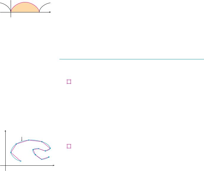
Even if C can’t be expressed in the form y F x , Formula 4 is still valid but we obtain it by polygonal approximations. We divide the parameter interval , into n subintervals of equal width t. If t0, t1, t2, . . . , tn are the endpoints of these subintervals, then xi f ti and yi t ti are the coordinates of points Pi xi, yi that lie on C and the polygon with vertices P0, P1 , . . . , Pn approximates C. (See Figure 4.)
As in Section 8.1, we define the length L of C to be the limit of the lengths of these approximating polygons as n l :
n
L lim Pi 1Pi
nl i 1
The Mean Value Theorem, when applied to f on the interval ti 1, ti , gives a number ti* in
ti 1, ti such that
f ti f ti 1 f ti* ti ti 1
If we let xi xi xi 1 and yi yi yi 1, this equation becomes
xi f ti* t

634 |||| CHAPTER 10 PARAMETRIC EQUATIONS AND POLAR COORDINATES
Similarly, when applied to t, the Mean Value Theorem gives a number ti** in ti 1, ti such that
yi t ti** t
Therefore
Pi 1Pi s xi 2 yi 2 s f ti* t 2 t ti** t 2
s f ti* 2 t ti** 2 t
and so
|
|
n |
|
|
|
|
L lim |
s |
|
|
t |
5 |
f ti* 2 |
t ti** 2 |
|||
|
n l |
|
|
|
|
|
|
i 1 |
|
|
|
The sum in (5) resembles a Riemann sum for the function s f t 2 t t 2 but it is not exactly a Riemann sum because ti* ti** in general. Nevertheless, if f and t are continuous, it can be shown that the limit in (5) is the same as if ti* and ti** were equal, namely,
L y s f t 2 t t 2 dt
Thus, using Leibniz notation, we have the following result, which has the same form as
Formula (4).
6 THEOREM If a curve C is described by the parametric equations x f t ,
y t t , t , where f and t are continuous on , and C is traversed
exactly once as t increases from |
to , then the length of C is |
||||||||||
|
y |
|
|
|
|
|
|
|
|
|
|
|
|
|
dx |
|
2 |
|
dy |
|
2 |
|
|
L |
|
|
|
|
|
|
dt |
||||
|
dt |
|
|
|
dt |
|
|
||||
|
|
|
|
|
|
|
|||||
Notice that the formula in Theorem 6 is consistent with the general formulas L xds and ds 2 dx 2 dy 2 of Section 8.1.
EXAMPLE 4 If we use the representation of the unit circle given in Example 2 in Section 10.1,
x cos t y sin t
0 t 2
then dx dt sin t and dy dt cos t, so Theorem 6 gives
|
y |
|
|
|
|
|
|
|
|
|
|
|
|
|
|
|
|
|
|
|
|
|
|
|
|
|
|
||
|
2 |
|
|
dx |
2 |
|
|
dy |
|
2 |
|
|
|
|
|
|
|
|
|
|
|
|
2 |
|
|
|
|||
L |
0 |
|
|
dt |
|
|
|
dt |
|
|
dt y0 |
ssin2t cos2t dt |
||
y2
0
dt 2
as expected. If, on the other hand, we use the representation given in Example 3 in Section 10.1,
x sin 2t y cos 2t
0
t 2
then dx dt 2 cos 2t, dy dt 2 sin 2t, and the integral in Theorem 6 gives
0 |
|
|
|
|
|
|
|
|
|
|
|
|
|
|
|
|
|
y |
|
|
dx |
|
2 |
|
dy |
|
2 |
|
|
|
|
|
|
|
|
2 |
|
|
|
|
|
|
|
|
|
|
|
|
|
||||
|
|
|
|
|
|
|
2 |
|
|
|
|
|
2 |
|
|||
|
|
|
dt |
|
|
|
dt |
|
|
dt y0 |
|
s4 cos2 |
2t 4 sin2 |
2t dt y0 |
2 dt 4 |
||
SECTION 10.2 CALCULUS WITH PARAMETRIC CURVES |||| 635
|Notice that the integral gives twice the arc length of the circle because as t increases from 0 to 2 , the point sin 2t, cos 2t traverses the circle twice. In general, when finding the length of a curve C from a parametric representation, we have to be careful to ensure
that C is traversed only once as t increases from to . |
M |
N The result of Example 5 says that the length of one arch of a cycloid is eight times the radius of the generating circle (see Figure 5). This was first proved in 1658 by Sir Christopher Wren, who later became the architect of St. Paul’s Cathedral in London.
y
L=8r
 r
r
02πr x
FIGURE 5
|
EXAMPLE 5 Find the length of one arch of the cycloid x r sin , |
|||||||||||||||||||||||||||
V |
||||||||||||||||||||||||||||
y r 1 cos |
. |
|
|
|
|
|
|
|
|
|
|
|
|
|
|
|
|
|
|
|
|
|
||||||
SOLUTION From Example 3 we see that one arch is described by the parameter interval |
||||||||||||||||||||||||||||
0 2 . Since |
|
|
|
|
|
|
|
|
|
|
|
|
|
|
|
|
|
|
|
|
|
|||||||
|
|
|
|
|
|
|
|
dx |
|
r 1 cos |
and |
|
dy |
r sin |
||||||||||||||
|
|
|
|
|
|
|
|
d |
|
|
|
|||||||||||||||||
|
|
|
|
|
|
|
|
|
|
|
|
|
|
|
|
|
|
|
|
|
d |
|
|
|
|
|||
we have |
|
|
|
|
|
|
|
|
|
|
|
|
|
|
|
|
|
|
|
|
|
|
|
|
|
|
||
|
|
|
|
|
|
|
|
|
|
|
|
|
|
|
|
|
|
|
|
|
|
|
|
|
|
|
||
|
|
|
|
|
|
|
|
|
|
|
|
|
|
|
|
|
|
|
|
|
|
|
|
|
|
|
||
|
|
|
|
|
|
|
|
|
|
|
|
|
|
|
|
|
|
|
|
|
|
|
|
|
|
|
||
|
|
y |
|
|
|
|
|
|
|
|
|
|
|
|
|
|
|
|
|
|
|
|
|
|||||
|
|
2 |
|
|
|
|
|
dx |
|
|
2 |
|
|
dy |
|
2 |
|
2 |
|
|
|
|
|
|
|
|
|
|
|
L |
0 |
|
|
|
|
|
d |
|
|
|
|
|
d |
|
|
d y0 |
sr2 1 |
cos |
2 r2 sin2 d |
||||||||
|
|
2 |
|
|
|
|
|
|
|
|
|
|
|
|
|
|
|
|
|
|
|
|
2 |
|
|
|
|
|
|
|
|
|
|
|
|
|
|
|
|
|
|
|
|
|
|
|
|
|
|
|
|
||||||
|
y0 |
|
sr2 1 |
2 cos |
cos2 sin2 d |
r y0 |
s2 1 cos d |
|||||||||||||||||||||
To evaluate this integral we use the identity sin2x 12 1 cos 2x with 2x, which
gives 1 cos 2 sin2 2 . Since 0 |
2 , we have 0 |
2 and so |
||||||||
sin 2 0. Therefore |
|
|
|
|
|
|
|
|||
|
s |
|
s |
|
2 sin 2 2 sin 2 |
|||||
|
2 1 cos |
4 sin2 2 |
||||||||
|
2 |
|
|
|
2r 2 cos 2 ] |
2 |
|
|||
and so |
|
L 2r y0 sin 2 d |
0 |
|
||||||
|
|
2r 2 2 8r |
|
|
|
|
M |
|||
SURFACE AREA
In the same way as for arc length, we can adapt Formula 8.2.5 to obtain a formula for surface area. If the curve given by the parametric equations x f t , y t t , t , is rotated about the x-axis, where f , t are continuous and t t 0, then the area of the resulting surface is given by
|
|
2 y |
dx |
2 |
|
dy |
|
2 |
7 |
S y |
|
|
|
|
|
dt |
|
dt |
dt |
The general symbolic formulas S x2 y ds and S x2 x ds (Formulas 8.2.7 and 8.2.8) are still valid, but for parametric curves we use
ds dxdt 2 dydt 2 dt
EXAMPLE 6 Show that the surface area of a sphere of radius r is 4 r2.
SOLUTION The sphere is obtained by rotating the semicircle
x r cos t y r sin t 0 t

636 |||| CHAPTER 10 PARAMETRIC EQUATIONS AND POLAR COORDINATES
about the x-axis. Therefore, from Formula 7, we get
|
|
|
|
|
|
|
|
|
|
|
|
|
|
||
|
|
|
|
S y0 2 r sin t s r sin t 2 r cos t 2 dt |
|||||||||||
|
|
|
|
|
|
|
|
|
|
|
|||||
|
|
|
|
|
2 y0 |
r sin t sr2 sin2t |
cos2t dt 2 y0 r sin t r dt |
||||||||
|
|
|
|
|
|
|
|
|
|
|
|
|
|
|
|
|
|
|
|
|
2 r2 |
y0 sin t dt 2 r2 cos t ]0 4 r2 |
|||||||||
|
|
|
|
|
|
|
|
|
|
|
|
|
|
|
|
|
10.2 |
EXERCISES |
|
|
|
|
|
|
|
|
|
|
|
|
|
|
|
|
|
|
|
|
|
|
|
|
|
|
|
|
|
1–2 Find dy dx. |
|
|
|
|
19. |
x 2 cos |
, |
y sin 2 |
|||||||
|
|
|
|
|
|
|
|||||||||
1. x t sin t, y t 2 t |
2. x 1 t, y s |
|
e t |
|
|
|
|
|
|
|
|
|
|||
t |
20. |
x cos 3 |
|
y 2 sin |
|
|
|||||||||
|
|
|
|
|
|
|
, |
|
|
||||||
M
3–6 Find an equation of the tangent to the curve at the point corresponding to the given value of the parameter.
3. |
x t 4 1, y t 3 t; t 1 |
|
4. |
x t t 1, y 1 t 2; t 1 |
|
5. |
x est , y t ln t 2; t 1 |
|
6. |
x cos sin 2 , y sin cos 2 ; |
0 |
|
|
|
7– 8 Find an equation of the tangent to the curve at the given point by two methods: (a) without eliminating the parameter and (b) by first eliminating the parameter.
7. |
x 1 ln t, y t 2 2; 1, 3 |
||
8. |
x tan , y sec ; (1, s |
|
) |
2 |
|||
|
|
|
|
;9–10 Find an equation of the tangent(s) to the curve at the given point. Then graph the curve and the tangent(s).
9. |
x 6 sin t, y t 2 t; 0, 0 |
10. |
x cos t cos 2t, y sin t sin 2t ; 1, 1 |
|
|
11–16 Find dy dx and d 2 y dx 2. For which values of t is the curve concave upward?
11. |
x 4 t 2, |
y t 2 t 3 |
12. |
x t 3 12t, |
y t 2 1 |
13. |
x t e t, |
y t e t |
14. |
x t ln t, |
y t ln t |
15. |
x 2 sin t, |
y 3 cos t, |
0 t 2 |
|
|
16. |
x cos 2t, |
y cos t, |
0 t |
|
|
|
|
|
|
|
|
17–20 Find the points on the curve where the tangent is horizontal or vertical. If you have a graphing device, graph the curve to check your work.
17. |
x 10 t 2, y t 3 12t |
18. |
x 2t 3 3t 2 12t, y 2t 3 3t 2 1 |
;21. Use a graph to estimate the coordinates of the rightmost point on the curve x t t 6, y e t. Then use calculus to find the exact coordinates.
;22. Use a graph to estimate the coordinates of the lowest point and the leftmost point on the curve x t 4 2t, y t t 4. Then find the exact coordinates.
;23–24 Graph the curve in a viewing rectangle that displays all the important aspects of the curve.
23. x t 4 |
2t 3 |
2t 2, |
y t 3 t |
24. x t 4 |
4t 3 |
8t 2, |
y 2t 2 t |
|
|
|
|
25.Show that the curve x cos t, y sin t cos t has two tangents at 0, 0 and find their equations. Sketch the curve.
;26. Graph the curve x cos t 2 cos 2t, y sin t 2 sin 2t to discover where it crosses itself. Then find equations of both tangents at that point.
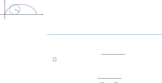
27.(a) Find the slope of the tangent line to the trochoid
x r d sin , y r d cos in terms of . (See Exercise 40 in Section 10.1.)
(b)Show that if d r, then the trochoid does not have a vertical tangent.
28. (a) Find the slope of the tangent to the astroid x a cos3 |
, |
y a sin3 in terms of . (Astroids are explored in the Laboratory Project on page 629.)
(b)At what points is the tangent horizontal or vertical?
(c)At what points does the tangent have slope 1 or 1?
29.At what points on the curve x 2t 3, y 1 4t t 2 does the tangent line have slope 1?
30. |
Find equations of the tangents to the curve x 3t 2 1, |
|
|
|
y 2t 3 1 that pass through the point 4, 3 . |
|
|
Use the parametric equations of an ellipse, x a cos , |
31. |
||
|
|
y b sin , 0 2 , to find the area that it encloses. |
32.Find the area enclosed by the curve x t 2 2t, y st and the y-axis.
33.Find the area enclosed by the x-axis and the curve
x1 e t, y t t 2.
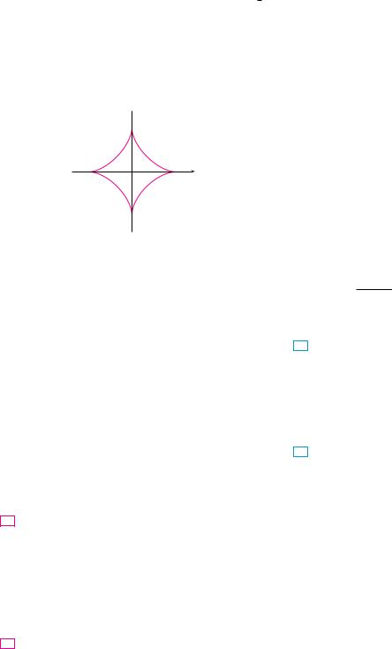
34.Find the area of the region enclosed by the astroid
xa cos3 , y a sin3 . (Astroids are explored in the Labo-
ratory Project on page 629.)
y a
a
_a |
0 |
a x |
_a
35.Find the area under one arch of the trochoid of Exercise 40 in Section 10.1 for the case d r.
36.Let be the region enclosed by the loop of the curve in Example 1.
(a)Find the area of .
(b)If is rotated about the x-axis, find the volume of the resulting solid.
(c)Find the centroid of .
37– 40 Set up an integral that represents the length of the curve. Then use your calculator to find the length correct to four decimal places.
37. |
x t t 2, |
y 34 t 3 2, |
1 t 2 |
|||||||
38. |
x 1 e t, |
y t 2, 3 t 3 |
||||||||
39. |
x t cos t, y t sin t, 0 t 2 |
|||||||||
40. |
x ln t, y s |
|
|
1 t 5 |
||||||
t 1, |
||||||||||
|
|
|
|
|
|
|
||||
|
|
41– 44 Find the exact length of the curve. |
||||||||
41. |
x 1 3t 2, |
y 4 2t 3, |
0 t 1 |
|||||||
42. |
x et e t, |
y 5 2t, |
0 t 3 |
|||||||
|
|
|
|
t |
y ln 1 t , |
0 t 2 |
||||
43. |
x |
|
, |
|||||||
1 t |
||||||||||
44. |
x 3 cos t cos 3t, y 3 sin t sin 3t, 0 t |
|||||||||
|
|
|
|
|
|
|
||||
; 45– 47 Graph the curve and find its length. |
||||||||||
45. |
x e t cos t, |
y e t sin t, |
0 t |
|||||||
46. |
x cos t ln(tan 21 t), |
y sin t, 4 t 3 4 |
||||||||
47. |
x e t t, |
y 4e t 2, |
8 t 3 |
|||||||
|
|
|
|
|
|
|
||||
48. |
Find the length of the loop of the curve x 3t t 3, |
|||||||||
|
|
|
y 3t 2. |
|
|
|
|
|
||
SECTION 10.2 CALCULUS WITH PARAMETRIC CURVES |||| 637
49.Use Simpson’s Rule with n 6 to estimate the length of the curve x t e t, y t e t, 6 t 6.
50.In Exercise 43 in Section 10.1 you were asked to derive the parametric equations x 2a cot , y 2a sin2 for the curve called the witch of Maria Agnesi. Use Simpson’s Rule
with n 4 to estimate the length of the arc of this curve given by 4 2.
51–52 Find the distance traveled by a particle with position x, y as t varies in the given time interval. Compare with the length of the curve.
51. |
x sin2t, |
y cos2t, |
0 t 3 |
52. |
x cos2t, |
y cos t, |
0 t 4 |
|
|
|
|
53.Show that the total length of the ellipse x a sin , y b cos , a b 0, is
L 4a y0 2 s1 e 2 sin2 |
d |
||
|
|
|
|
where e is the eccentricity of the ellipse (e c a, where
c sa 2 b 2 ).
54.Find the total length of the astroid x a cos3 , y a sin3 , where a 0.
CAS 55. (a) Graph the epitrochoid with equations
x11 cos t 4 cos 11t 2
y11 sin t 4 sin 11t 2
What parameter interval gives the complete curve?
(b)Use your CAS to find the approximate length of this curve.
CAS 56. A curve called Cornu’s spiral is defined by the parametric equations
t |
|
x C t y0 |
cos u 2 2 du |
t |
|
y S t y0 |
sin u 2 2 du |
where C and S are the Fresnel functions that were introduced in Chapter 5.
(a)Graph this curve. What happens as t l and as t l ?
(b)Find the length of Cornu’s spiral from the origin to the point with parameter value t.
57–58 Set up an integral that represents the area of the surface obtained by rotating the given curve about the x-axis. Then use your calculator to find the surface area correct to four decimal places.
57. |
x 1 te t, y t 2 1 e t, 0 t 1 |
58. |
x sin2t, y sin 3t, 0 t 3 |
|
|
638 |||| CHAPTER 10 PARAMETRIC EQUATIONS AND POLAR COORDINATES
59–61 Find the exact area of the surface obtained by rotating the given curve about the x-axis.
59. |
x t 3, y t 2, 0 t 1 |
|
|
60. |
x 3t t 3, |
y 3t 2, 0 t 1 |
|
61. |
x a cos3 , |
y a sin3 , 0 |
2 |
|
|
|
|
; 62. Graph the curve
x 2 cos cos 2 |
y 2 sin sin 2 |
If this curve is rotated about the x-axis, find the area of the resulting surface. (Use your graph to help find the correct parameter interval.)
63. If the curve |
|
||
x t t 3 y t |
1 |
1 t 2 |
|
t 2 |
|||
|
|
||
is rotated about the x-axis, use your calculator to estimate the area of the resulting surface to three decimal places.
64.If the arc of the curve in Exercise 50 is rotated about the x-axis, estimate the area of the resulting surface using Simpson’s Rule with n 4.
65–66 Find the surface area generated by rotating the given curve about the y-axis.
65. |
x 3t 2, y 2t 3, 0 t 5 |
66. |
x e t t, y 4e t 2, 0 t 1 |
|
|
67.If f is continuous and f t 0 for a t b, show that the parametric curve x f t , y t t , a t b, can be put in the form y F x . [Hint: Show that f 1 exists.]
68.Use Formula 2 to derive Formula 7 from Formula 8.2.5 for
the case in which the curve can be represented in the form y F x , a x b.
69.The curvature at a point P of a curve is defined as
|
|
ds |
|
|
d |
|
|
where is the angle of inclination of the tangent line at P, as shown in the figure. Thus the curvature is the absolute value of the rate of change of with respect to arc length. It can be regarded as a measure of the rate of change of direction of the curve at P and will be studied in greater detail in Chapter 13.
(a)For a parametric curve x x t , y y t , derive the formula
xy x y
x 2 y 2 3 2
where the dots indicate derivatives with respect to t, so
x dx dt. [Hint: Use tan 1 dy dx and Formula 2 to find d dt. Then use the Chain Rule to find d ds.]
(b) By regarding a curve y f x as the parametric curve
x x, y f x , with parameter x, show that the formula in part (a) becomes
|
|
d 2 y dx 2 |
|
|
1 dy dx 2 3 2 |
||
|
y |
|
|
|
|
|
P |
˙
0x
70.(a) Use the formula in Exercise 69(b) to find the curvature of the parabola y x 2 at the point 1, 1 .
(b)At what point does this parabola have maximum curvature?
71.Use the formula in Exercise 69(a) to find the curvature of the
cycloid x sin , y 1 cos at the top of one of its arches.
72. (a) Show that the curvature at each point of a straight line is 0.
(b) Show that the curvature at each point of a circle of radius r is 1 r.
73.A string is wound around a circle and then unwound while being held taut. The curve traced by the point P at the end of the string is called the involute of the circle. If the circle has
radius r and center O and the initial position of P is r, 0 ,
and if the parameter |
is chosen as in the figure, show |
|||
that parametric equations of the involute are |
|
|||
x r cos |
sin |
y r sin |
|
cos |
|
y |
|
|
|
|
|
T |
|
|
|
r |
P |
|
|
|
¨ |
|
|
|
|
O |
|
x |
|
74. A cow is tied to a silo with radius r by a rope just long enough to reach the opposite side of the silo. Find the area available for grazing by the cow.