

- •CONTENTS
- •Preface
- •To the Student
- •Diagnostic Tests
- •1.1 Four Ways to Represent a Function
- •1.2 Mathematical Models: A Catalog of Essential Functions
- •1.3 New Functions from Old Functions
- •1.4 Graphing Calculators and Computers
- •1.6 Inverse Functions and Logarithms
- •Review
- •2.1 The Tangent and Velocity Problems
- •2.2 The Limit of a Function
- •2.3 Calculating Limits Using the Limit Laws
- •2.4 The Precise Definition of a Limit
- •2.5 Continuity
- •2.6 Limits at Infinity; Horizontal Asymptotes
- •2.7 Derivatives and Rates of Change
- •Review
- •3.2 The Product and Quotient Rules
- •3.3 Derivatives of Trigonometric Functions
- •3.4 The Chain Rule
- •3.5 Implicit Differentiation
- •3.6 Derivatives of Logarithmic Functions
- •3.7 Rates of Change in the Natural and Social Sciences
- •3.8 Exponential Growth and Decay
- •3.9 Related Rates
- •3.10 Linear Approximations and Differentials
- •3.11 Hyperbolic Functions
- •Review
- •4.1 Maximum and Minimum Values
- •4.2 The Mean Value Theorem
- •4.3 How Derivatives Affect the Shape of a Graph
- •4.5 Summary of Curve Sketching
- •4.7 Optimization Problems
- •Review
- •5 INTEGRALS
- •5.1 Areas and Distances
- •5.2 The Definite Integral
- •5.3 The Fundamental Theorem of Calculus
- •5.4 Indefinite Integrals and the Net Change Theorem
- •5.5 The Substitution Rule
- •6.1 Areas between Curves
- •6.2 Volumes
- •6.3 Volumes by Cylindrical Shells
- •6.4 Work
- •6.5 Average Value of a Function
- •Review
- •7.1 Integration by Parts
- •7.2 Trigonometric Integrals
- •7.3 Trigonometric Substitution
- •7.4 Integration of Rational Functions by Partial Fractions
- •7.5 Strategy for Integration
- •7.6 Integration Using Tables and Computer Algebra Systems
- •7.7 Approximate Integration
- •7.8 Improper Integrals
- •Review
- •8.1 Arc Length
- •8.2 Area of a Surface of Revolution
- •8.3 Applications to Physics and Engineering
- •8.4 Applications to Economics and Biology
- •8.5 Probability
- •Review
- •9.1 Modeling with Differential Equations
- •9.2 Direction Fields and Euler’s Method
- •9.3 Separable Equations
- •9.4 Models for Population Growth
- •9.5 Linear Equations
- •9.6 Predator-Prey Systems
- •Review
- •10.1 Curves Defined by Parametric Equations
- •10.2 Calculus with Parametric Curves
- •10.3 Polar Coordinates
- •10.4 Areas and Lengths in Polar Coordinates
- •10.5 Conic Sections
- •10.6 Conic Sections in Polar Coordinates
- •Review
- •11.1 Sequences
- •11.2 Series
- •11.3 The Integral Test and Estimates of Sums
- •11.4 The Comparison Tests
- •11.5 Alternating Series
- •11.6 Absolute Convergence and the Ratio and Root Tests
- •11.7 Strategy for Testing Series
- •11.8 Power Series
- •11.9 Representations of Functions as Power Series
- •11.10 Taylor and Maclaurin Series
- •11.11 Applications of Taylor Polynomials
- •Review
- •APPENDIXES
- •A Numbers, Inequalities, and Absolute Values
- •B Coordinate Geometry and Lines
- •E Sigma Notation
- •F Proofs of Theorems
- •G The Logarithm Defined as an Integral
- •INDEX
608 |||| CHAPTER 9 DIFFERENTIAL EQUATIONS
liter. In order to reduce the concentration of chlorine, fresh water is pumped into the tank at a rate of 4 L s. The mixture is kept stirred and is pumped out at a rate of 10 L s. Find the amount of chlorine in the tank as a function of time.
35.An object with mass m is dropped from rest and we assume that the air resistance is proportional to the speed of the object.
If s t is the distance dropped after t seconds, then the speed is v s t and the acceleration is a v t . If t is the acceleration due to gravity, then the downward force on the object is mt cv, where c is a positive constant, and Newton’s Second Law gives
mdv mt cv dt
(a)Solve this as a linear equation to show that
vmt 1 e ct m
c
(b)What is the limiting velocity?
(c)Find the distance the object has fallen after t seconds.
36.If we ignore air resistance, we can conclude that heavier objects fall no faster than lighter objects. But if we take air resistance into account, our conclusion changes. Use the
expression for the velocity of a falling object in Exercise 35(a) to find dv dm and show that heavier objects do fall faster than lighter ones.
9.6 PREDATOR-PREY SYSTEMS
We have looked at a variety of models for the growth of a single species that lives alone in an environment. In this section we consider more realistic models that take into account the interaction of two species in the same habitat. We will see that these models take the form of a pair of linked differential equations.
We first consider the situation in which one species, called the prey, has an ample food supply and the second species, called the predator, feeds on the prey. Examples of prey and predators include rabbits and wolves in an isolated forest, food fish and sharks, aphids and ladybugs, and bacteria and amoebas. Our model will have two dependent variables and both are functions of time. We let R t be the number of prey (using R for rabbits) and W t be the number of predators (with W for wolves) at time t.
In the absence of predators, the ample food supply would support exponential growth of the prey, that is,
dR kR where k is a positive constant dt
In the absence of prey, we assume that the predator population would decline at a rate proportional to itself, that is,
dW rW where r is a positive constant dt
With both species present, however, we assume that the principal cause of death among the prey is being eaten by a predator, and the birth and survival rates of the predators depend on their available food supply, namely, the prey. We also assume that the two species encounter each other at a rate that is proportional to both populations and is therefore proportional to the product RW. (The more there are of either population, the more encounters there are likely to be.) A system of two differential equations that incorporates these assumptions is as follows:
1 |
dR kR aRW |
dW rW bRW |
||
W represents the predator. |
|
|
|
|
R represents the prey. |
dt |
dt |
||
where k, r, a, and b are positive constants. Notice that the term aRW decreases the natural growth rate of the prey and the term bRW increases the natural growth rate of the predators.

N The Lotka-Volterra equations were proposed as a model to explain the variations in the shark and food-fish populations in the Adriatic Sea
by the Italian mathematician Vito Volterra (1860–1940).
SECTION 9.6 PREDATOR-PREY SYSTEMS |||| 609
The equations in (1) are known as the predator-prey equations, or the Lotka-Volterra equations. A solution of this system of equations is a pair of functions R t and W t that describe the populations of prey and predator as functions of time. Because the system is coupled (R and W occur in both equations), we can’t solve one equation and then the other; we have to solve them simultaneously. Unfortunately, it is usually impossible to find explicit formulas for R and W as functions of t. We can, however, use graphical methods to analyze the equations.
V EXAMPLE 1 Suppose that populations of rabbits and wolves are described by the Lotka-Volterra equations (1) with k 0.08, a 0.001, r 0.02, and b 0.00002. The time t is measured in months.
(a)Find the constant solutions (called the equilibrium solutions) and interpret the answer.
(b)Use the system of differential equations to find an expression for dW dR.
(c)Draw a direction field for the resulting differential equation in the RW-plane. Then use that direction field to sketch some solution curves.
(d)Suppose that, at some point in time, there are 1000 rabbits and 40 wolves. Draw the corresponding solution curve and use it to describe the changes in both population levels.
(e)Use part (d) to make sketches of R and W as functions of t.
SOLUTION
(a) With the given values of k, a, r, and b, the Lotka-Volterra equations become
dR 0.08R 0.001RW dt
dW 0.02W 0.00002RW dt
Both R and W will be constant if both derivatives are 0, that is,
R R 0.08 0.001W 0
W W 0.02 0.00002R 0
One solution is given by R 0 and W 0. (This makes sense: If there are no rabbits or wolves, the populations are certainly not going to increase.) The other constant solution is
W |
0.08 |
80 |
R |
0.02 |
1000 |
|
|
||||
0.001 |
|
0.00002 |
|
||
So the equilibrium populations consist of 80 wolves and 1000 rabbits. This means that 1000 rabbits are just enough to support a constant wolf population of 80. There are neither too many wolves (which would result in fewer rabbits) nor too few wolves (which would result in more rabbits).
(b) We use the Chain Rule to eliminate t:
|
|
|
|
|
|
|
|
|
dW |
|
dW |
|
dR |
|
|
|
|
|
|
|
|
|
|
|
|
|
|
||||
|
|
|
|
|
|
|
|
|
dt dR dt |
||||||
|
|
|
|
|
dW |
|
|
|
|
|
|
|
|
|
|
|
dW |
|
|
|
|
|
|
|
|
0.02W 0.00002RW |
|||||
so |
|
|
dt |
|
|
|
|||||||||
|
dR dR |
|
|
|
|
0.08R 0.001RW |
|||||||||
|
|
|
|
|
|
|
|
|
|
|
|
|
|
|
|
dt

610 |||| CHAPTER 9 DIFFERENTIAL EQUATIONS
(c) If we think of W as a function of R, we have the differential equation
dW 0.02W 0.00002RW dR 0.08R 0.001RW
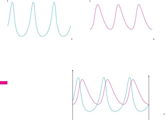
We draw the direction field for this differential equation in Figure 1 and we use it to sketch several solution curves in Figure 2. If we move along a solution curve, we observe how the relationship between R and W changes as time passes. Notice that the curves appear to be closed in the sense that if we travel along a curve, we always return to the same point. Notice also that the point (1000, 80) is inside all the solution curves. That point is called an equilibrium point because it corresponds to the equilibrium solution R 1000, W 80.
W |
|
|
|
W |
|
|
|
150 |
|
|
|
150 |
|
|
|
100 |
|
|
|
100 |
|
|
|
50 |
|
|
|
50 |
|
|
|
0 |
1000 |
2000 |
3000 R |
0 |
1000 |
2000 |
3000 R |
FIGURE 1 |
Direction field for the predator-prey system |
FIGURE 2 |
Phase portrait of the system |
|
|||
FIGURE 3
Phase trajectory through (1000,40)
When we represent solutions of a system of differential equations as in Figure 2, we refer to the RW-plane as the phase plane, and we call the solution curves phase trajectories. So a phase trajectory is a path traced out by solutions R, W as time goes by. A phase portrait consists of equilibrium points and typical phase trajectories, as shown in Figure 2.
(d) Starting with 1000 rabbits and 40 wolves corresponds to drawing the solution curve through the point P0 1000, 40 . Figure 3 shows this phase trajectory with the direction field removed. Starting at the point P0 at time t 0 and letting t increase, do we move clockwise or counterclockwise around the phase trajectory? If we put R 1000 and
W |
|
P™ |
|
|
|
|
|
140 |
|
|
|
|
|
|
|
|
|
|
|
|
|
|
|
120 |
|
|
|
|
|
|
|
100 |
|
|
|
|
|
|
|
80 |
P£ |
|
|
|
|
P¡ |
|
60 |
|
|
|
|
|
|
|
40 |
|
P¸(1000,40) |
|
|
|
|
|
|
|
|
|
|
|
||
20 |
|
|
|
|
|
|
|
0 |
500 |
1000 |
1500 |
2000 |
2500 |
3000 |
R |
|
|
|
|
|
|
|
|
|
|
|
|
|
|
|
|
|
|
|
|
|
|
|
|
|
SECTION 9.6 |
PREDATOR-PREY SYSTEMS |||| 611 |
|
|
|
|
|
|
|
|
|
|
|
|
W 40 in the first differential equation, we get |
|
|
||||||||||||||
|
|
|
|
|
|
|
|
|
|
|
|
|
dR |
0.08 1000 0.001 1000 40 80 40 40 |
|||||||||||||
|
|
|
|
|
|
|
|
|
|
|
|
|
|
||||||||||||||
|
|
|
|
|
|
|
|
|
|
|
|
|
dt |
|
|
||||||||||||
|
|
|
|
|
|
|
|
|
|
|
Since dR dt 0, we conclude that R is increasing at P0 and so we move counter- |
||||||||||||||||
|
|
|
|
|
|
|
|
|
|
|
clockwise around the phase trajectory. |
|
|
||||||||||||||
|
|
|
|
|
|
|
|
|
|
|
We see that at P0 there aren’t enough wolves to maintain a balance between the popu- |
||||||||||||||||
|
|
|
|
|
|
|
|
|
|
|
lations, so the rabbit population increases. That results in more wolves and eventually |
||||||||||||||||
|
|
|
|
|
|
|
|
|
|
|
there are so many wolves that the rabbits have a hard time avoiding them. So the number |
||||||||||||||||
|
|
|
|
|
|
|
|
|
|
|
of rabbits begins to decline (at P1, where we estimate that R reaches its maximum popu- |
||||||||||||||||
|
|
|
|
|
|
|
|
|
|
|
lation of about 2800). This means that at some later time the wolf population starts to |
||||||||||||||||
|
|
|
|
|
|
|
|
|
|
|
fall (at P2, where R 1000 and W 140). But this benefits the rabbits, so their popula- |
||||||||||||||||
|
|
|
|
|
|
|
|
|
|
|
tion later starts to increase (at P3, where W 80 and R 210). As a consequence, the |
||||||||||||||||
|
|
|
|
|
|
|
|
|
|
|
wolf population eventually starts to increase as well. This happens when the populations |
||||||||||||||||
|
|
|
|
|
|
|
|
|
|
|
return to their initial values of R 1000 and W 40, and the entire cycle begins again. |
||||||||||||||||
|
|
|
|
|
|
|
|
|
|
|
(e) From the description in part (d) of how the rabbit and wolf populations rise and fall, |
||||||||||||||||
|
|
|
|
|
|
|
|
|
|
|
we can sketch the graphs of R t and W t . Suppose the points P1, P2, and P3 in Figure 3 |
||||||||||||||||
|
|
|
|
|
|
|
|
|
|
|
are reached at times t1, t2, and t3. Then we can sketch graphs of R and W as in Figure 4. |
||||||||||||||||
R |
|
|
|
|
|
|
W |
|
|
|
|
||||||||||||||||
|
|
|
|
|
|
|
|
||||||||||||||||||||
2500 |
|
|
|
|
|
|
|
|
|
|
|
|
140 |
|
|
|
|
|
|
|
|
|
|
|
|
||
|
|
|
|
|
|
|
|
|
|
|
|
|
|
|
|
|
|
|
|
|
|
|
|
||||
|
|
|
|
|
|
|
|
|
|
|
|
120 |
|
|
|
|
|
|
|
|
|
|
|
|
|||
2000 |
|
|
|
|
|
|
|
|
|
|
|
|
|
|
|
|
|
|
|
|
|
|
|
|
|||
|
|
|
|
|
|
|
|
|
|
|
|
|
|
|
|
|
|
|
|
|
|
|
|
||||
|
|
|
|
|
|
|
|
|
|
|
|
100 |
|
|
|
|
|
|
|
|
|
|
|
|
|||
|
|
|
|
|
|
|
|
|
|
|
|
|
|
|
|
|
|
|
|
|
|
|
|
||||
|
|
|
|
|
|
|
|
|
|
|
|
|
|
|
|
|
|
|
|
|
|
|
|
|
|||
1500 |
|
|
|
|
|
|
|
|
|
|
|
|
80 |
|
|
|
|
|
|
|
|
|
|
|
|
||
|
|
|
|
|
|
|
|
|
|
|
|
|
|
|
|
|
|||||||||||
1000 |
|
|
|
|
|
|
|
|
|
|
|
|
60 |
|
|
|
|
|
|
|
|
|
|
|
|
||
|
|
|
|
|
|
|
|
|
|
|
|
|
|
|
|
|
|
|
|
|
|
|
|
||||
|
|
|
|
|
|
|
|
|
|
|
|
40 |
|
|
|
|
|
|
|
|
|
|
|
|
|||
500 |
|
|
|
|
|
|
|
|
|
|
|
|
|
|
|
|
|
|
|
|
|
|
|
|
|||
|
|
|
|
|
|
|
|
|
|
|
|
|
|
|
|
|
|
|
|
|
|
|
|
||||
|
|
|
|
|
|
|
|
|
|
|
|
20 |
|
|
|
|
|
|
|
|
|
|
|
|
|||
|
|
|
|
|
|
|
|
|
|
|
|
|
|
|
|
|
|
|
|
|
|
|
|
||||
|
|
|
|
|
|
|
|
|
|
|
|
|
|
|
|
|
|
|
|
|
|
|
|
|
|||
|
|
|
|
|
|
|
|
|
|
|
|
|
|
|
|
|
|
|
|
|
|
|
|
|
|
|
|
0 |
|
t¡ t™ t£ |
t |
|
|
0 |
|
t¡ t™ t£ |
t |
||||||||||||||||||
|
|
|
|
|
|
|
|
|
|
|
|
|
|
|
|
|
|
|
|
||||||||
FIGURE 4 |
|
|
|
|
|
|
|
|
|
|
|
|
|
|
|
|
|
||||||||||
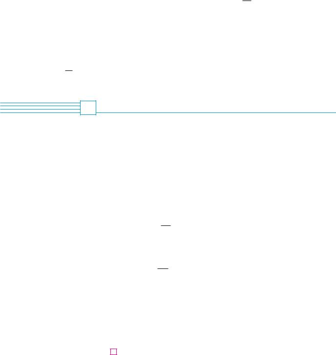
Graphs of the rabbit and wolf |
To make the graphs easier to compare, we draw the graphs on the same axes but with |
||||||||||||||||||||||||||
populations as functions of time |
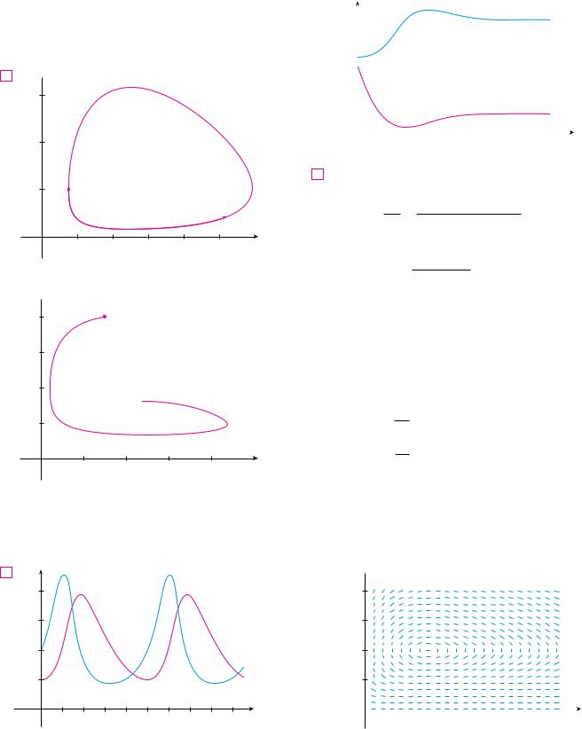
different scales for R and W, as in Figure 5. Notice that the rabbits reach their maximum |
||||||||||||||||||||||||||
|
|
|
|
|
|
|
|
|
|
|
populations about a quarter of a cycle before the wolves. |
||||||||||||||||
TEC In Module 9.6 you can change the coefficients in the Lotka-Volterra equations and observe the resulting changes in the phase trajectory and graphs of the rabbit and wolf populations.
FIGURE 5
Comparison of the rabbit and wolf populations
|
R |
|
|
|
|
|
|
|
|
|
|
|
|
|
3000 |
|
|
|
|
|
|
|
|
|
|
|
W |
||
|
|
|
|
|
|
|
|
|
|
|
||||
|
|
|
|
|
|
|
|
|
|
|
|
|
||
|
|
|
|
|
|
|
|
|
|
|
R |
|||
|
|
|
|
|
|
|
|
|
|
|
W |
|||
Number 2000 |
|
|
|
|
|
|
|
|
|
|
|
120 |
|
|
|
|
|
|
|
|
|
|
|
|
|
||||
|
|
|
|
|
|
|
|
|
|
|
Number |
|||
|
|
|
|
|
|
|
|
|
|
|
||||
|
of |
|
|
|
|
|
|
|
|
|
|
|
of |
|
|
rabbits |
|
|
|
|
|
|
|
|
|
|
|
80 wolves |
|
|
|
|
|
|
|
|
|
|
|
|
|
|||
1000 |
|
|
|
|
|
|
|
|
|
|
|
40 |
|
|
|
|
|
|
|
|
|
|
|
|
|
|
|||
|
|
|
|
|
|
|
|
|
|
|
|
|
|
|
|
|
|
|
|
|
|
|
|
|
|
|
|
||
|
|
|
|
|
|
|
|
|
|
|
|
|
|
|
|
0 |
|
t¡ t™ |
t£ |
|
|
t |
|||||||
M
612 |||| CHAPTER 9 DIFFERENTIAL EQUATIONS
FIGURE 6
Relative abundance of hare and lynx from Hudson’s Bay Company records
An important part of the modeling process, as we discussed in Section 1.2, is to interpret our mathematical conclusions as real-world predictions and to test the predictions against real data. The Hudson’s Bay Company, which started trading in animal furs in Canada in 1670, has kept records that date back to the 1840s. Figure 6 shows graphs of the number of pelts of the snowshoe hare and its predator, the Canada lynx, traded by the company over a 90-year period. You can see that the coupled oscillations in the hare and lynx populations predicted by the Lotka-Volterra model do actually occur and the period of these cycles is roughly 10 years.
|
160 |
|
|
|
|
|
|
|
|
hare |
|
|
|
|
120 |
|
|
|
9 |
|
|
|
|
|
|
|
|
|
|
|
lynx |
|
|
|
Thousands |
80 |
|
|
|
6 |
Thousands |
of hares |
|
|
|
|
of lynx |
|
|
40 |
|
|
|
3 |
|
|
0 |
1850 |
1875 |
1900 |
1925 |
|
Although the relatively simple Lotka-Volterra model has had some success in explaining and predicting coupled populations, more sophisticated models have also been proposed. One way to modify the Lotka-Volterra equations is to assume that, in the absence of predators, the prey grow according to a logistic model with carrying capacity K. Then the Lotka-Volterra equations (1) are replaced by the system of differential equations
dR |
kR |
|
1 |
R |
|
aRW |
dW |
rW bRW |
|
|
K |
|
|
||||
dt |
|
|
dt |
|||||
This model is investigated in Exercises 9 and 10.
Models have also been proposed to describe and predict population levels of two species that compete for the same resources or cooperate for mutual benefit. Such models are explored in Exercise 2.
9.6E X E R C I S E S
1.For each predator-prey system, determine which of the variables, x or y, represents the prey population and which represents the predator population. Is the growth of the prey restricted just by the predators or by other factors as well? Do the predators feed only on the prey or do they have additional food sources? Explain.
(a)dx 0.05x 0.0001xy dt
dy 0.1y 0.005xy dt
(b)dx 0.2x 0.0002x2 0.006xy dt
dy 0.015y 0.00008xy dt
2.Each system of differential equations is a model for two species that either compete for the same resources or cooperate for mutual benefit (flowering plants and insect pollinators, for instance). Decide whether each system describes competition or cooperation and explain why it is a reasonable model. (Ask yourself what effect an increase in one species has on the growth rate of the other.)
(a)dx 0.12x 0.0006x2 0.00001xy dt
dy 0.08x 0.00004xy dt
(b)dx 0.15x 0.0002x2 0.0006xy dt
dy 0.2y 0.00008y2 0.0002xy
dt
3– 4 A phase trajectory is shown for populations of rabbits R and foxes F .
(a)Describe how each population changes as time goes by.
(b)Use your description to make a rough sketch of the graphs of R and F as functions of time.
3. F
300
200 |
|
|
|
|
|
|
100 |
t=0 |
|
|
|
|
|
0 |
400 |
800 |
1200 |
1600 |
2000 |
R |
4.F
160 |
t=0 |
120
80
40
0 |
400 |
800 |
1200 |
1600 |
R |
|
|
|
|
|
|
5–6 Graphs of populations of two species are shown. Use them to sketch the corresponding phase trajectory.
5. |
y |
species 1 |
|
|
|
|
200 |
|
species 2
150
100
50
0 |
1 |
t |
|
|
|
|
SECTION 9.6 |
PREDATOR-PREY SYSTEMS |
|||| |
613 |
|||||||
6. |
y |
|
|
|
|
species 1 |
|
|
|
|
|
|||
|
|
|
|
|
|
|
|
|
|
|
|
|||
|
1200 |
|
|
|
|
|
|
|
|
|
|
|
|
|
|
|
|
|
|
|
|
|
|
|
|
|
|
|
|
|
1000 |
|
|
|
|
|
|
|
|
|
|
|
|
|
|
|
|
|
|
|
|
|
|
|
|
|
|
|
|
|
|
|
|
|
|
|
|
|
|
|
|
|
|
|
|
800 |
|
|
|
|
|
|
|
|
|
|
|
|
|
|
|
|
|
|
|
|
|
|
|
|
|
|
|
|
|
|
|
|
|
|
|
|
|
|
|
|
|
|
|
|
600 |
|
|
|
|
|
|
|
|
|
|
|
|
|
|
|
|
|
|
|
|
|
|
|
|
|
|
|
|
|
|
|
|
|
|
|
|
|
|
|
|
|
|
|
|
400 |
|
|
|
|
|
species 2 |
|
|
|
|
|
||
|
|
|
|
|
|
|
|
|
|
|
||||
|
|
|
|
|
|
|
|
|
|
|
||||
|
200 |
|
|
|
|
|
|
|
|
|
|
|||
|
|
|
|
|
|
|
|
|
|
|
||||
|
|
|
|
|
|
|
|
|
|
|
|
|
|
|
|
|
|
|
|
|
|
|
|
|
|
|
|
|
|
|
|
|
|
|
|
|
|
|
|
|
|
|
|
|
|
|
|
|
|
|
|
|
|
|
|
|
|
|
|
|
0 |
|
5 |
10 |
15 |
t |
||||||||
|
|
|
|
|
|
|
|
|
|
|
|
|
|
|
7.In Example 1(b) we showed that the rabbit and wolf populations satisfy the differential equation
dW 0.02W 0.00002RW dR 0.08R 0.001RW
By solving this separable differential equation, show that
R0.02W 0.08
e 0.00002Re 0.001W C
where C is a constant.
It is impossible to solve this equation for W as an explicit function of R (or vice versa). If you have a computer algebra system that graphs implicitly defined curves, use this equation and your CAS to draw the solution curve that passes through the point 1000, 40 and compare with Figure 3.
8.Populations of aphids and ladybugs are modeled by the equations
dA 2A 0.01AL dt
dL 0.5L 0.0001AL dt
(a)Find the equilibrium solutions and explain their significance.
(b)Find an expression for dL dA.
(c)The direction field for the differential equation in part (b) is shown. Use it to sketch a phase portrait. What do the phase trajectories have in common?
L 400
400
300
200
100
0 |
|
|
|
|
|
|
|
5000 |
10000 |
15000 A |
|||||