9.4 MODELS FOR POPULATION GROWTH

Добавил:

PavelEngineer Опубликованный материал нарушает ваши авторские права? Сообщите нам.

Вуз:

Севастопольский Государственный Университет

Предмет:

[НЕСОРТИРОВАННОЕ]

Файл:

[James_Stewart]_Single_Variable_Calculus_Early_Tr(BookFi).pdf

Скачиваний:

Добавлен:

30.12.2019

Размер:

18.09 Mб

Скачать

☆

<<< < Предыдущая 52 53 54 55 56 57 58 59 60 61 62 6364 / 9164 65 66 67 68 69 70 71 72 73 74 75 76 > Следующая >>>

SECTION 9.4 MODELS FOR POPULATION GROWTH |||| 591

tial equation

In this section we investigate differential equations that are used to model population growth: the law of natural growth, the logistic equation, and several others.

THE LAW OF NATURAL GROWTH

One of the models for population growth that we considered in Section 9.1 was based on the assumption that the population grows at a rate proportional to the size of the population:

dP kP dt

Is that a reasonable assumption? Suppose we have a population (of bacteria, for instance) with size P 1000 and at a certain time it is growing at a rate of P 300 bacteria per hour. Now let’s take another 1000 bacteria of the same type and put them with the ﬁrst population. Each half of the new population was growing at a rate of 300 bacteria per hour. We would expect the total population of 2000 to increase at a rate of 600 bacteria per hour initially (provided there’s enough room and nutrition). So if we double the size, we double the growth rate. In general, it seems reasonable that the growth rate should be proportional to the size.

In general, if P t is the value of a quantity y at time t and if the rate of change of P with respect to t is proportional to its size P t at any time, then

1	dP	kP

	dt

N Examples and exercises on the use of (2) are given in Section 3.8.

where k is a constant. Equation 1 is sometimes called the law of natural growth. If k is positive, then the population increases; if k is negative, it decreases.

Because Equation 1 is a separable differential equation, we can solve it by the methods of Section 9.3:

y dPP yk dt ln P kt C

P ekt C eCekt

P Aekt

where A ( eC or 0) is an arbitrary constant. To see the signiﬁcance of the constant A, we observe that

P 0 Aek 0 A

Therefore A is the initial value of the function.

2 The solution of the initial-value problem
	dP	kP	P 0 P0
		kP	P 0 P0
	dt
is		P t P0ekt

592 |||| CHAPTER 9 DIFFERENTIAL EQUATIONS

Another way of writing Equation 1 is

1 dP k P dt

which says that the relative growth rate (the growth rate divided by the population size) is constant. Then (2) says that a population with constant relative growth rate must grow exponentially.

We can account for emigration (or “harvesting”) from a population by modifying Equation 1: If the rate of emigration is a constant m, then the rate of change of the population is modeled by the differential equation

3	dP	kP m

	dt

See Exercise 13 for the solution and consequences of Equation 3.

THE LOGISTIC MODEL

As we discussed in Section 9.1, a population often increases exponentially in its early stages but levels off eventually and approaches its carrying capacity because of limited resources. If P t is the size of the population at time t, we assume that

dP	kP	if P is small

dt

This says that the growth rate is initially close to being proportional to size. In other words, the relative growth rate is almost constant when the population is small. But we also want to reﬂect the fact that the relative growth rate decreases as the population P increases and becomes negative if P ever exceeds its carrying capacity K, the maximum population that the environment is capable of sustaining in the long run. The simplest expression for the relative growth rate that incorporates these assumptions is

1	dP	k	1	P
P				K
	dt

Multiplying by P, we obtain the model for population growth known as the logistic differential equation:

4	dP	kP	1	P
				K
	dt

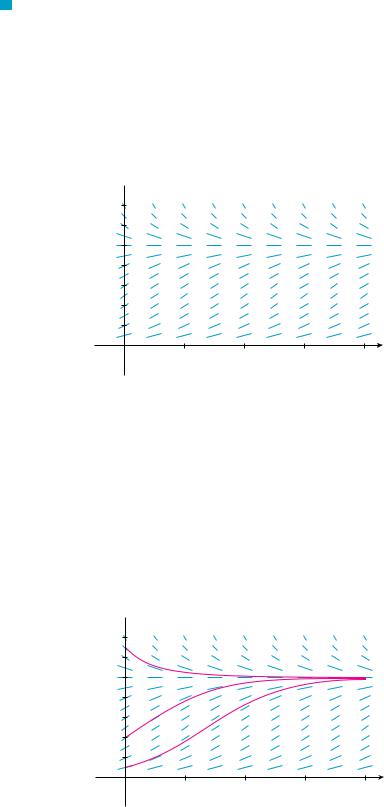
Notice from Equation 4 that if P is small compared with K, then P K is close to 0 and so dP dt kP. However, if P l K (the population approaches its carrying capacity), then P K l 1, so dP dt l 0. We can deduce information about whether solutions increase or decrease directly from Equation 4. If the population P lies between 0 and K, then the right side of the equation is positive, so dP dt 0 and the population increases. But if the population exceeds the carrying capacity P K , then 1 P K is negative, so dP dt 0 and the population decreases.

Let’s start our more detailed analysis of the logistic differential equation by looking at a direction ﬁeld.

SECTION 9.4 MODELS FOR POPULATION GROWTH |||| 593

FIGURE 1

Direction field for the logistic equation in Example 1

V EXAMPLE 1 Draw a direction ﬁeld for the logistic equation with k 0.08 and carrying capacity K 1000. What can you deduce about the solutions?

SOLUTION In this case the logistic differential equation is

dP	0.08P	1	P
			1000
dt

A direction ﬁeld for this equation is shown in Figure 1. We show only the ﬁrst quadrant because negative populations aren’t meaningful and we are interested only in what happens after t 0.

P 1400 1200 1000 800 600 400 200

80 t

The logistic equation is autonomous (dP dt depends only on P, not on t), so the slopes are the same along any horizontal line. As expected, the slopes are positive for 0 P 1000 and negative for P 1000.

The slopes are small when P is close to 0 or 1000 (the carrying capacity). Notice that the solutions move away from the equilibrium solution P 0 and move toward the equilibrium solution P 1000.

In Figure 2 we use the direction ﬁeld to sketch solution curves with initial populations P 0 100, P 0 400, and P 0 1300. Notice that solution curves that start below P 1000 are increasing and those that start above P 1000 are decreasing. The slopes are greatest when P 500 and therefore the solution curves that start below P 1000 have inﬂection points when P 500. In fact we can prove that all solution curves that start below P 500 have an inﬂection point when P is exactly 500. (See Exercise 9.)

FIGURE 2

Solution curves for the logistic equation in Example 1

P 1400 1200 1000 800 600 400 200

80 t

594 |||| CHAPTER 9 DIFFERENTIAL EQUATIONS

The logistic equation (4) is separable and so we can solve it explicitly using the method

of Section 9.3. Since

we have

yk dt

P 1 P K

To evaluate the integral on the left side, we write

P 1 P K

P K P

Using partial fractions (see Section 7.4), we get

P K P

K P

This enables us to rewrite Equation 5:

dP yk dt

K P

ln P ln K P kt C

K P

kt C

K P

e kt C e Ce kt

K P

Ae kt

where A e C. Solving Equation 6 for P, we get

1 Ae kt

Ae kt

1 Ae kt

We ﬁnd the value of A by putting t 0 in Equation 6. If t 0, then P P0 (the initial population), so

K P0 Ae0 A

N Compare the solution curve in Figure 3 with the lowest solution curve we drew from the direction ﬁeld in Figure 2.

1000

P=900

1000 P=1+9e_0.08t

FIGURE 3

	SECTION 9.4		MODELS FOR POPULATION GROWTH \|\|\|\| 595
Thus the solution to the logistic equation is

7	P t	K	where A	K P0
7	P t	Ae kt	where A	P0
	1	Ae kt		P0

Using the expression for P t in Equation 7, we see that

lim P t K

t l

which is to be expected.

EXAMPLE 2 Write the solution of the initial-value problem

dP	0.08P	1	P	P 0 100
			1000
dt

and use it to ﬁnd the population sizes P 40 and P 80 . At what time does the population reach 900?

SOLUTION The differential equation is a logistic equation with k 0.08, carrying capacity K 1000, and initial population P0 100. So Equation 7 gives the population at time t as


P t			1000		where A	1000 100		9
P t			1 Ae 0.08t		where A		100	9
Thus				P t	1000

					1 9e 0.08t
So the population sizes when t 40 and 80 are
P 40		1000		731.6	P 80		1000		985.3

	1 9e 3.2						1 9e 6.4

The population reaches 900 when

1000

1 9e 0.08t 900

Solving this equation for t, we get

1 9e 0.08t 109 e 0.08t 811

0.08t ln 811 ln 81

t ln 81 54.9 0.08

So the population reaches 900 when t is approximately 55. As a check on our work, we graph the population curve in Figure 3 and observe where it intersects the line P 900. The cursor indicates that t 55. M

596 |||| CHAPTER 9 DIFFERENTIAL EQUATIONS

COMPARISON OF THE NATURAL GROWTH AND LOGISTIC MODELS

In the 1930s the biologist G. F. Gause conducted an experiment with the protozoan Paramecium and used a logistic equation to model his data. The table gives his daily count of the population of protozoa. He estimated the initial relative growth rate to be 0.7944 and the carrying capacity to be 64.

t (days)	0	1	2	3	4	5	6	7	8	9	10	11	12	13	14	15	16

P (observed)	2	3	22	16	39	52	54	47	50	76	69	51	57	70	53	59	57

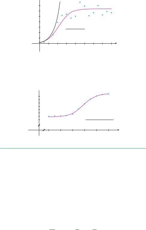
V EXAMPLE 3 Find the exponential and logistic models for Gause’s data. Compare the predicted values with the observed values and comment on the ﬁt.

SOLUTION Given the relative growth rate k 0.7944 and the initial population P0 2, the exponential model is

P t P0 ekt 2e0.7944t

Gause used the same value of k for his logistic model. [This is reasonable because

P0 2 is small compared with the carrying capacity (K 64). The equation

1	dP	t 0	k	1	2	k
P0	dt
				64

shows that the value of k for the logistic model is very close to the value for the exponential model.]

Then the solution of the logistic equation in Equation 7 gives

								P t			K						64
								P t			Ae		kt				Ae			0.7944t
								1			Ae			1			Ae
			where						A	K P0					64 2				31
			where						A										31
											P0			2
			So						P t					64

												1 31e 0.7944t
			We use these equations to calculate the predicted values (rounded to the nearest integer)
			and compare them in the following table.

t (days)	0	1	2	3	4	5	6		7		8		9			10		11			12	13	14	15	16

P (observed)	2	3	22	16	39	52	54		47		50		76			69		51			57	70	53	59	57

P (logistic model)	2	4	9	17	28	40	51		57		61		62			63		64			64	64	64	64	64

P (exponential model)	2	4	10	22	48	106	. . .

We notice from the table and from the graph in Figure 4 that for the ﬁrst three or four days the exponential model gives results comparable to those of the more sophisticated logistic model. For t 5, however, the exponential model is hopelessly inaccurate, but the logistic model ﬁts the observations reasonably well.

KP 1 mP

FIGURE 4

The exponential and logistic models for the Paramecium data

t	B t	t	B t

1980	9,847	1992	10,036
1982	9,856	1994	10,109
1984	9,855	1996	10,152
1986	9,862	1998	10,175
1988	9,884	2000	10,186
1990	9,962

FIGURE 5

Logistic model for the population of Belgium

SECTION 9.4 MODELS FOR POPULATION GROWTH |||| 597

P=2e0.7944t

20 P=1+31e_0.7944t

16 t

Many countries that formerly experienced exponential growth are now ﬁnding that their rates of population growth are declining and the logistic model provides a better model. The table in the margin shows midyear values of B t , the population of Belgium, in thousands, at time t, from 1980 to 2000. Figure 5 shows these data points together with a shifted logistic function obtained from a calculator with the ability to ﬁt a logistic function to these points by regression. We see that the logistic model provides a very good ﬁt.

10,100

10,000

9,900

350

9,800 P=9840+1+2.05e_0.48(t-1990)

0	1980	1984	1988	1992	1996	2000	t

OTHER MODELS FOR POPULATION GROWTH

The Law of Natural Growth and the logistic differential equation are not the only equations that have been proposed to model population growth. In Exercise 18 we look at the Gompertz growth function and in Exercises 19 and 20 we investigate seasonal-growth models.

Two of the other models are modiﬁcations of the logistic model. The differential

equation
	dP	kP	1	P	c
				K
	dt

has been used to model populations that are subject to harvesting of one sort or another. (Think of a population of ﬁsh being caught at a constant rate.) This equation is explored in Exercises 15 and 16.

For some species there is a minimum population level m below which the species tends to become extinct. (Adults may not be able to ﬁnd suitable mates.) Such populations have been modeled by the differential equation

dP kP 1 dt

where the extra factor, 1 m P, takes into account the consequences of a sparse population (see Exercise 17).

598 |||| CHAPTER 9 DIFFERENTIAL EQUATIONS

9.4		EXERCISES
					where y t is the biomass (the total mass of the members of
1.	Suppose that a population develops according to the logistic				where y t is the biomass (the total mass of the members of
	equation				the population) in kilograms at time t (measured in years), the
			dP	0.05P 0.0005P 2	carrying capacity is estimated to be K 8 107 kg, and
			dt	0.05P 0.0005P 2	k 0.71 per year.
			dt		k 0.71 per year.
	where t is measured in weeks.				(a) If y 0 2 107 kg, ﬁnd the biomass a year later.
	where t is measured in weeks.				(b) How long will it take for the biomass to reach 4 107 kg?
	(a) What is the carrying capacity? What is the value of k?
	(b) A direction ﬁeld for this equation is shown. Where are				4. The table gives the number of yeast cells in a new laboratory
		the slopes close to 0? Where are they largest? Which			culture.
		solutions are increasing? Which solutions are decreasing?

P 150

100

60 t

(c)Use the direction ﬁeld to sketch solutions for initial populations of 20, 40, 60, 80, 120, and 140. What do these solutions have in common? How do they differ? Which solutions have inﬂection points? At what population levels do they occur?

(d)What are the equilibrium solutions? How are the other solutions related to these solutions?

;2. Suppose that a population grows according to a logistic model with carrying capacity 6000 and k 0.0015 per year.

(a)Write the logistic differential equation for these data.

(b)Draw a direction ﬁeld (either by hand or with a computer algebra system). What does it tell you about the solution curves?

(c)Use the direction ﬁeld to sketch the solution curves for initial populations of 1000, 2000, 4000, and 8000. What can you say about the concavity of these curves? What is the signiﬁcance of the inﬂection points?

(d)Program a calculator or computer to use Euler’s method with step size h 1 to estimate the population after

50 years if the initial population is 1000.

(e)If the initial population is 1000, write a formula for the population after t years. Use it to ﬁnd the population after 50 years and compare with your estimate in part (d).

(f)Graph the solution in part (e) and compare with the solution curve you sketched in part (c).

3. The Paciﬁc halibut ﬁshery has been modeled by the differen-

Time (hours)	Yeast cells	Time (hours)	Yeast cells

0	18	10	509
2	39	12	597
4	80	14	640
6	171	16	664
8	336	18	672

(a)Plot the data and use the plot to estimate the carrying capacity for the yeast population.

(b)Use the data to estimate the initial relative growth rate.

(c)Find both an exponential model and a logistic model for these data.

(d)Compare the predicted values with the observed values, both in a table and with graphs. Comment on how well your models ﬁt the data.

(e)Use your logistic model to estimate the number of yeast cells after 7 hours.

5.The population of the world was about 5.3 billion in 1990. Birth rates in the 1990s ranged from 35 to 40 million per year and death rates ranged from 15 to 20 million per year. Let’s assume that the carrying capacity for world population is

100 billion.

(a)Write the logistic differential equation for these data. (Because the initial population is small compared to the carrying capacity, you can take k to be an estimate of the initial relative growth rate.)

(b)Use the logistic model to estimate the world population in the year 2000 and compare with the actual population of 6.1 billion.

(c)Use the logistic model to predict the world population in the years 2100 and 2500.

(d)What are your predictions if the carrying capacity is 50 billion?

6.(a) Make a guess as to the carrying capacity for the US population. Use it and the fact that the population was 250 million in 1990 to formulate a logistic model for the US population.

(b)Determine the value of k in your model by using the fact that the population in 2000 was 275 million.

(c)Use your model to predict the US population in the years 2100 and 2200.

SECTION 9.4 MODELS FOR POPULATION GROWTH |||| 599

(d)Use your model to predict the year in which the US population will exceed 350 million.

7.One model for the spread of a rumor is that the rate of spread is proportional to the product of the fraction y of the population who have heard the rumor and the fraction who have not heard the rumor.

(a)Write a differential equation that is satisﬁed by y.

(b)Solve the differential equation.

(c)A small town has 1000 inhabitants. At 8 AM, 80 people have heard a rumor. By noon half the town has heard it. At what time will 90% of the population have heard the rumor?

8.Biologists stocked a lake with 400 ﬁsh and estimated the carrying capacity (the maximal population for the ﬁsh of that species in that lake) to be 10,000. The number of ﬁsh tripled in the ﬁrst year.

(a)Assuming that the size of the ﬁsh population satisﬁes the logistic equation, ﬁnd an expression for the size of the population after t years.

(b)How long will it take for the population to increase to 5000?

9.(a) Show that if P satisﬁes the logistic equation (4), then

dt 2	k 2P 1 K 1		K
d 2P		P	2P

(b)Deduce that a population grows fastest when it reaches half its carrying capacity.

;10. For a ﬁxed value of K (say K 10), the family of logistic functions given by Equation 7 depends on the initial value P0 and the proportionality constant k. Graph several members of this family. How does the graph change when P0 varies? How does it change when k varies?

;11. The table gives the midyear population of Japan, in thousands, from 1960 to 2005.

Year	Population	Year	Population

1960	94,092	1985	120,754
1965	98,883	1990	123,537
1970	104,345	1995	125,341
1975	111,573	2000	126,700
1980	116,807	2005	127,417

Use a graphing calculator to ﬁt both an exponential function and a logistic function to these data. Graph the data points and both functions, and comment on the accuracy of the models. [Hint: Subtract 94,000 from each of the population ﬁgures. Then, after obtaining a model from your calculator, add 94,000 to get your ﬁnal model. It might be helpful to choose t 0 to correspond to 1960 or 1980.]

;12.The table gives the midyear population of Spain, in thousands, from 1955 to 2000.

Year	Population	Year	Population

1955	29,319	1980	37,488
1960	30,641	1985	38,535
1965	32,085	1990	39,351
1970	33,876	1995	39,750
1975	35,564	2000	40,016

Use a graphing calculator to ﬁt both an exponential function and a logistic function to these data. Graph the data points and both functions, and comment on the accuracy of the models. [Hint: Subtract 29,000 from each of the population ﬁgures. Then, after obtaining a model from your calculator, add 29,000 to get your ﬁnal model. It might be helpful to choose t 0 to correspond to 1955 or 1975.]

13. Consider a population P P t with constant relative birth and death rates and , respectively, and a constant emigration rate m, where , , and m are positive constants. Assume

that	. Then the rate of change of the population at time
t is modeled by the differential equation
		dP	kP m	where k

		dt

(a)Find the solution of this equation that satisﬁes the initial condition P 0 P0.

(b)What condition on m will lead to an exponential expansion of the population?

(c)What condition on m will result in a constant population? A population decline?

(d)In 1847, the population of Ireland was about 8 million and the difference between the relative birth and death rates was 1.6% of the population. Because of the potato famine in the 1840s and 1850s, about 210,000 inhabitants per year emigrated from Ireland. Was the population expanding or declining at that time?

14.Let c be a positive number. A differential equation of the form

dy ky 1 c dt

where k is a positive constant, is called a doomsday equation because the exponent in the expression ky 1 c is larger than the exponent 1 for natural growth.

(a) Determine the solution that satisﬁes the initial condition y 0 y0.

(b) Show that there is a ﬁnite time t T (doomsday) such that lim t lT y t .

(c) An especially proliﬁc breed of rabbits has the growth term ky 1.01. If 2 such rabbits breed initially and the warren has 16 rabbits after three months, then when is doomsday?

600 |||| CHAPTER 9 DIFFERENTIAL EQUATIONS

15. Let’s modify the logistic differential equation of Example 1

as follows:
	dP	0.08P	1	P	15
				1000
	dt

(a)Suppose P t represents a ﬁsh population at time t, where t is measured in weeks. Explain the meaning of the term 15.

(b)Draw a direction ﬁeld for this differential equation.

(c)What are the equilibrium solutions?

(d)Use the direction ﬁeld to sketch several solution curves.

Describe what happens to the ﬁsh population for various initial populations.

CAS (e) Solve this differential equation explicitly, either by using partial fractions or with a computer algebra system. Use the initial populations 200 and 300. Graph the solutions and compare with your sketches in part (d).

CAS 16. Consider the differential equation

dP	0.08P	1	P	c
			1000
dt

as a model for a ﬁsh population, where t is measured in weeks and c is a constant.

(a)Use a CAS to draw direction ﬁelds for various values of c.

(b)From your direction ﬁelds in part (a), determine the values of c for which there is at least one equilibrium solution. For what values of c does the ﬁsh population always die out?

(c)Use the differential equation to prove what you discovered graphically in part (b).

(d)What would you recommend for a limit to the weekly catch of this ﬁsh population?

17.There is considerable evidence to support the theory that for some species there is a minimum population m such that the species will become extinct if the size of the population falls

below m. This condition can be incorporated into the logistic equation by introducing the factor 1 m P . Thus the modiﬁed logistic model is given by the differential equation

dt			K		P
dP	kP	1	P	1	m

(a)Use the differential equation to show that any solution is increasing if m P K and decreasing if 0 P m.

(b)For the case where k 0.08, K 1000, and m 200, draw a direction ﬁeld and use it to sketch several solution curves. Describe what happens to the population for various initial populations. What are the equilibrium solutions?

(c)Solve the differential equation explicitly, either by using partial fractions or with a computer algebra system. Use the initial population P0 .

(d)Use the solution in part (c) to show that if P0 m, then

the species will become extinct. [Hint: Show that the numerator in your expression for P t is 0 for some value of t.]

18.Another model for a growth function for a limited population is given by the Gompertz function, which is a solution of the differential equation

dP c ln K P dt P

where c is a constant and K is the carrying capacity.

(a)Solve this differential equation.

(b)Compute lim t l P t .

(c)Graph the Gompertz growth function for K 1000,

P0 100, and c 0.05, and compare it with the logistic function in Example 2. What are the similarities? What are the differences?

(d)We know from Exercise 9 that the logistic function grows fastest when P K 2. Use the Gompertz differential

equation to show that the Gompertz function grows fastest when P K e.

19.In a seasonal-growth model, a periodic function of time is introduced to account for seasonal variations in the rate of growth. Such variations could, for example, be caused by seasonal changes in the availability of food.

(a)Find the solution of the seasonal-growth model

		dP	kP cos rt	P 0 P0

		dt
;	where k, r, and are positive constants.
	(b) By graphing the solution for several values of k, r, and ,
	explain how the values of k, r, and affect the solution.
	What can you say about lim t l P t ?

20.Suppose we alter the differential equation in Exercise 19 as follows:

		dP	kP cos2 rt	P 0 P0

		dt
	(a) Solve this differential equation with the help of a table of
;	integrals or a CAS.
	(b) Graph the solution for several values of k, r, and . How
	do the values of k, r, and affect the solution? What can
	you say about lim t l P t in this case?

21.Graphs of logistic functions (Figures 2 and 3) look suspiciously similar to the graph of the hyperbolic tangent function (Figure 3 in Section 3.11). Explain the similarity by showing that the logistic function given by Equation 7 can be written as

P t 12 K[1 tanh(12 k t c )]

where c ln A k. Thus the logistic function is really just a shifted hyperbolic tangent.

APPLIED PROJECT CALCULUS AND BASEBALL |||| 601

A P P L I E D	CALCULUS AND BASEBALL
P R O J E C T	In this project we explore three of the many applications of calculus to baseball. The physical

	interactions of the game, especially the collision of ball and bat, are quite complex and their
	models are discussed in detail in a book by Robert Adair, The Physics of Baseball, 3d ed.
	(New York: HarperPerennial, 2002).
	1. It may surprise you to learn that the collision of baseball and bat lasts only about a thou-
	sandth of a second. Here we calculate the average force on the bat during this collision by
	ﬁrst computing the change in the ball’s momentum.
	The momentum p of an object is the product of its mass m and its velocity v, that is,
	p mv. Suppose an object, moving along a straight line, is acted on by a force F F t
	that is a continuous function of time.
	(a) Show that the change in momentum over a time interval t0, t1 is equal to the integral
	of F from t0 to t1; that is, show that
		t1
Batter’s box		p t1 p t0 yt0	F t dt

	This integral is called the impulse of the force over the time interval.
	(b) A pitcher throws a 90-mi h fastball to a batter, who hits a line drive directly back
	to the pitcher. The ball is in contact with the bat for 0.001 s and leaves the bat with
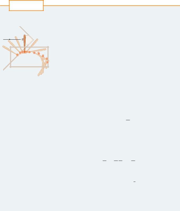
An overhead view of the position of a	velocity 110 mi h. A baseball weighs 5 oz and, in US Customary units, its mass is
	measured in slugs: m w t where t 32 ft s2.
baseball bat, shown every ﬁftieth of	(i)	Find the change in the ball’s momentum.
a second during a typical swing.
	(ii)	Find the average force on the bat.
(Adapted from The Physics of Baseball)

2.In this problem we calculate the work required for a pitcher to throw a 90-mi h fastball by

ﬁrst considering kinetic energy.

The kinetic energy K of an object of mass m and velocity v is given by K 12 mv2. Suppose an object of mass m, moving in a straight line, is acted on by a force F F s that depends on its position s. According to Newton’s Second Law

F s ma m dv dt

where a and v denote the acceleration and velocity of the object.

(a)Show that the work done in moving the object from a position s0 to a position s1 is equal to the change in the object’s kinetic energy; that is, show that

W y1 F s ds 12 mv12 12 mv02

where v0 v s0 and v1 v s1 are the velocities of the object at the positions s0 and s1. Hint: By the Chain Rule,

m dv m dv ds mv dv dt ds dt ds

(b)How many foot-pounds of work does it take to throw a baseball at a speed of 90 mi h?

3.(a) An outﬁelder ﬁelds a baseball 280 ft away from home plate and throws it directly to the catcher with an initial velocity of 100 ft s. Assume that the velocity v t of the ball after t seconds satisﬁes the differential equation dv dt 101 v because of air resistance. How long does it take for the ball to reach home plate? (Ignore any vertical motion of the ball.)

(b)The manager of the team wonders whether the ball will reach home plate sooner if it is relayed by an inﬁelder. The shortstop can position himself directly between the out-

ﬁelder and home plate, catch the ball thrown by the outﬁelder, turn, and throw the ball to

<<< < Предыдущая 52 53 54 55 56 57 58 59 60 61 62 6364 / 9164 65 66 67 68 69 70 71 72 73 74 75 76 > Следующая >>>

Соседние файлы в предмете [НЕСОРТИРОВАННОЕ]

#
05.02.202055.36 Mб21Calculus, 7th Edition ( PDFDrive.com ).pdf
#
30.12.201945.82 Mб43Complete Solutions Manual for_ SINGLE VARIABLE CALCULUS Early Transcendentals 7th Edition by Stewart ( PDFDrive.com ).pdf
#
30.12.201918.09 Mб38[James_Stewart]_Single_Variable_Calculus_Early_Tr(BookFi).pdf