Добавил:

PavelEngineer Опубликованный материал нарушает ваши авторские права? Сообщите нам.

Вуз:

Севастопольский Государственный Университет

Предмет:

[НЕСОРТИРОВАННОЕ]

Файл:

[James_Stewart]_Single_Variable_Calculus_Early_Tr(BookFi).pdf

Скачиваний:

Добавлен:

30.12.2019

Размер:

18.09 Mб

Скачать

☆

<<< < Предыдущая 27 28 29 30 31 32 33 34 35 36 37 3839 / 9139 40 41 42 43 44 45 46 47 48 49 50 51 > Следующая >>>

400 |||| CHAPTER 5 INTEGRALS

2.Carl Boyer, The History of the Calculus and Its Conceptual Development (New York: Dover, 1959), Chapter V.

3.C. H. Edwards, The Historical Development of the Calculus (New York: Springer-Verlag, 1979), Chapters 8 and 9.

4.Howard Eves, An Introduction to the History of Mathematics, 6th ed. (New York: Saunders, 1990), Chapter 11.

5.C. C. Gillispie, ed., Dictionary of Scientiﬁc Biography (New York: Scribner’s, 1974).

See the article on Leibniz by Joseph Hofmann in Volume VIII and the article on Newton by I. B. Cohen in Volume X.

6.Victor Katz, A History of Mathematics: An Introduction (New York: HarperCollins, 1993), Chapter 12.

7.Morris Kline, Mathematical Thought from Ancient to Modern Times (New York: Oxford University Press, 1972), Chapter 17.

Sourcebooks

1.John Fauvel and Jeremy Gray, eds., The History of Mathematics: A Reader (London: MacMillan Press, 1987), Chapters 12 and 13.

2.D. E. Smith, ed., A Sourcebook in Mathematics (New York: Dover, 1959), Chapter V.

3.D. J. Struik, ed., A Sourcebook in Mathematics, 1200–1800 (Princeton, N.J.: Princeton University Press, 1969), Chapter V.

5.5 THE SUBSTITUTION RULE

N Differentials were deﬁned in Section 3.10. If u ! f ! x", then

du ! f #! x" dx

Because of the Fundamental Theorem, it’s important to be able to ﬁnd antiderivatives. But our antidifferentiation formulas don’t tell us how to evaluate integrals such as

	y2xs		dx
1		1 ' x2

To ﬁnd this integral we use the problem-solving strategy of introducing something extra. Here the “something extra” is a new variable; we change from the variable x to a new variable u. Suppose that we let u be the quantity under the root sign in (1), u ! 1 ' x2. Then the differential of u is du ! 2x dx. Notice that if the dx in the notation for an integral were to be interpreted as a differential, then the differential 2x dx would occur in (1) and so, formally, without justifying our calculation, we could write

	y2xs		dx ! ys		2x dx ! ys		du
2		1 ' x2		1 ' x2		u

! 23 u3#2 ' C ! 23 !x2 ' 1"3#2 ' C

But now we can check that we have the correct answer by using the Chain Rule to differentiate the ﬁnal function of Equation 2:

dxd [23 ! x2 ' 1"3#2 ' C] ! 23 ! 32 ! x2 ' 1"1#2 ! 2x ! 2xsx2 ' 1

In general, this method works whenever we have an integral that we can write in the form xf ! t! x"" t#!x" dx. Observe that if F# ! f, then

3	yF#! t! x""t#!x" dx ! F! t! x"" ' C

		SECTION 5.5 THE SUBSTITUTION RULE \|\|\|\| 401
because, by the Chain Rule,
	d	$F! t! x""% ! F#! t!x"" t#! x"
	dx	$F! t! x""% ! F#! t!x"" t#! x"

If we make the “change of variable” or “substitution” u ! t! x", then from Equation 3 we have

yF#! t! x"" t#! x" dx ! F! t! x"" ' C ! F!u" ' C ! yF#!u" du

or, writing F# ! f, we get

yf ! t! x"" t#! x" dx ! yf !u" du

Thus we have proved the following rule.

4 THE SUBSTITUTION RULE If u ! t!x" is a differentiable function whose range is an interval I and f is continuous on I, then

yf ! t! x"" t#! x" dx ! yf !u" du

Notice that the Substitution Rule for integration was proved using the Chain Rule for differentiation. Notice also that if u ! t! x", then du ! t#! x" dx, so a way to remember the Substitution Rule is to think of dx and du in (4) as differentials.

Thus the Substitution Rule says: It is permissible to operate with dx and du after integral signs as if they were differentials.

N Check the answer by differentiating it.

EXAMPLE 1 Find yx3 cos! x4 ' 2" dx.

SOLUTION We make the substitution u ! x4 ' 2 because its differential is du ! 4x3 dx, which, apart from the constant factor 4, occurs in the integral. Thus, using x3 dx ! du#4 and the Substitution Rule, we have

yx3 cos! x4 ' 2" dx ! ycos u ! 14 du ! 14 ycos u du

!14 sin u ' C

!14 sin! x4 ' 2" ' C

Notice that at the ﬁnal stage we had to return to the original variable x.

The idea behind the Substitution Rule is to replace a relatively complicated integral by a simpler integral. This is accomplished by changing from the original variable x to a new variable u that is a function of x. Thus, in Example 1, we replaced the integral xx3 cos! x4 ' 2" dx by the simpler integral 14 xcos u du.

The main challenge in using the Substitution Rule is to think of an appropriate substitution. You should try to choose u to be some function in the integrand whose differential also occurs (except for a constant factor). This was the case in Example 1. If that is not

402 |||| CHAPTER 5 INTEGRALS

©=- Ä!dx

FIGURE 1

Ä= x Пгггггг1-4≈

©=j Ä!dx=_ 41 Пгггггг1-4≈

possible, try choosing u to be some complicated part of the integrand (perhaps the inner function in a composite function). Finding the right substitution is a bit of an art. It’s not unusual to guess wrong; if your ﬁrst guess doesn’t work, try another substitution.

EXAMPLE 2 Evaluate ys

dx.

2x ' 1

SOLUTION 1

Let u ! 2x ' 1. Then du ! 2 dx, so dx ! du#2. Thus the Substitution Rule

gives

dx ! ys

du2 ! 21 yu1#2 du

2x ' 1

u3#2

' C !

3 u3#2 ' C

3#2

! 31 !2x ' 1"3#2 ' C

SOLUTION 2

Another possible substitution is u !

2x ' 1. Then

du !

dx !

du ! u du

2x ' 1

s2x ' 1

(Or observe that u2 ! 2x ' 1, so 2u du ! 2 dx.) Therefore

ys2x ' 1 dx ! yu ! u du ! yu2 du

' C ! 31 !2x ' 1"3#2 ' C

EXAMPLE 3 Find y

dx.

1 !

4x2

SOLUTION Let u ! 1 ! 4x2. Then du ! !8x dx, so x dx ! !81 du and

dx ! !81 y

du ! !81

yu!1#2 du

1 !

4x2

! !81 (2

u ) ' C ! !41 1 ! 4x2 ' C

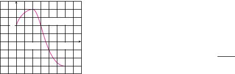
The answer to Example 3 could be checked by differentiation, but instead let’s check

it with a graph. In		Figure 1 we have used a computer to graph both the integrand
f ! x" ! x#s		and its indeﬁnite integral t!x" ! !41 s		(we take the case
	1 ! 4x2		1 ! 4x2

C ! 0). Notice that t! x" decreases when f ! x" is negative, increases when f !x" is positive, and has its minimum value when f ! x" ! 0. So it seems reasonable, from the graphical evidence, that t is an antiderivative of f.

EXAMPLE 4 Calculate ye5x dx.
SOLUTION If we let u ! 5x, then du ! 5 dx, so dx ! 51 du. Therefore
ye5x dx ! 51 yeu du ! 51 eu ' C ! 51 e5x ' C	M

SECTION 5.5 THE SUBSTITUTION RULE |||| 403

EXAMPLE 5 Find ys1 ' x2 x5 dx.

SOLUTION An appropriate substitution becomes more obvious if we factor x5 as x4 ! x. Let u ! 1 ' x2. Then du ! 2x dx, so x dx ! du#2. Also x2 ! u ! 1, so x4 ! !u ! 1"2:

ys1 ' x2 x5 dx ! ys1 ' x2 x4 ( x dx

!ysu !u ! 1"2 du2 ! 12 ysu !u2 ! 2u ' 1" du

!12 y!u5#2 ! 2u3#2 ' u1#2 " du

!12 (27 u7#2 ! 2 ( 25 u5#2 ' 23 u3#2 ) ' C

! 17 !1 ' x2 "7#2 ! 25 !1 ' x2 "5#2 ' 13 !1 ' x2 "3#2 ' C M

V EXAMPLE 6 Calculate ytan x dx.
SOLUTION First we write tangent in terms of sine and cosine:
ytan x dx ! y cossin xx dx
This suggests that we should substitute u ! cos x, since then du ! !sin x dx and so
sin x dx ! !du:
ytan x dx ! y cossin xx dx ! !y duu
! !ln ( u ( ' C ! !ln ( cos x ( ' C	M

Since !ln ( cos x ( ! ln!( cos x (!1" ! ln!1#(cos x (" ! ln ( sec x (, the result of Example 6 can also be written as

5	ytan x dx ! ln ( sec x ( ' C

DEFINITE INTEGRALS

When evaluating a deﬁnite integral by substitution, two methods are possible. One method is to evaluate the indeﬁnite integral ﬁrst and then use the Fundamental Theorem. For instance, using the result of Example 2, we have

y04 s2x ' 1 dx ! ys2x ' 1 dx]40 ! 13 !2x ' 1"3#2]40

! 13 !9"3#2 ! 13 !1"3#2 ! 13 !27 ! 1" ! 263

Another method, which is usually preferable, is to change the limits of integration when the variable is changed.

404 |||| CHAPTER 5 INTEGRALS

N This rule says that when using a substitution in a deﬁnite integral, we must put everything in terms of the new variable u, not only x and dx but also the limits of integration. The new limits of integration are the values of u that correspond to x ! a and x ! b.

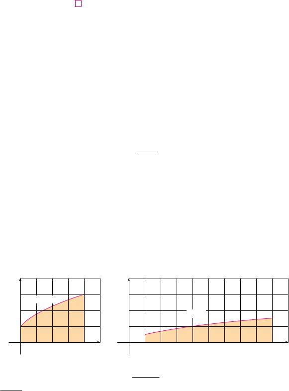
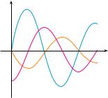
N The geometric interpretation of Example 7 is shown in Figure 2. The substitution u ! 2x " 1 stretches the interval $0, 4% by a factor of 2 and translates it to the right by 1 unit. The Substitution Rule shows that the two areas are equal.

6	THE SUBSTITUTION RULE FOR DEFINITE INTEGRALS If t# is continuous on
$a, b% and f is continuous on the range of u ! t"x#, then
	yab f " t"x##t#"x# dx ! ytt""ab## f "u# du

PROOF	Let F be an antiderivative of f. Then, by (3), F" t"x## is an antiderivative of
f " t"x##t#"x#, so by Part 2 of the Fundamental Theorem, we have
	yab f " t"x##t#"x# dx ! F" t"x##]ab ! F" t"b## ! F" t"a##
But, applying FTC2 a second time, we also have
	ytt""ab## f "u# du ! F"u#]tt""ab## ! F" t"b## ! F" t"a##	M

EXAMPLE 7 Evaluate y04 s2x " 1 dx using (6).

SOLUTION Using the substitution from Solution 1 of Example 2, we have u ! 2x " 1 and dx ! du!2. To ﬁnd the new limits of integration we note that


when x ! 0, u ! 2"0# " 1 ! 1				and			when x ! 4, u ! 2"4# " 1 ! 9
Therefore	y04 s		dx ! y19		21 s		du ! 21 ! 32 u3!2]19
Therefore	y04 s	2x " 1	dx ! y19		21 s	u	du ! 21 ! 32 u3!2]19
				! 31 "93!2 ! 13!2 # ! 263
Observe that when using (6) we do not return to the variable x after integrating. We
simply evaluate the expression in u between the appropriate values of u.								M

y
3	y=Пггггг2x+1
	y=Пггггг2x+1
2
1
0	4	x
FIGURE 2

y
3
2		y=	Ïãu
			2
1
0	1		9	u

N The integral given in Example 8 is an abbreviation for

y12 "3 !15x#2 dx

y2 dx

EXAMPLE 8 Evaluate 1 "3 ! 5x#2 .

SOLUTION Let u ! 3 ! 5x. Then du ! !5 dx, so dx ! !du!5. When x ! 1, u ! !2 and

SECTION 5.5 THE SUBSTITUTION RULE |||| 405

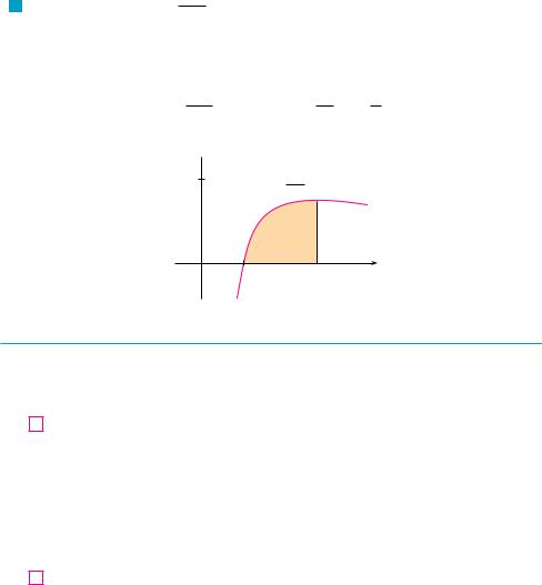
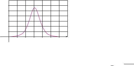
N Since the function f "x# ! "ln x#!x in Example 9 is positive for x $ 1, the integral represents the area of the shaded region in Figure 3.

FIGURE 3

when x ! 2, u ! !7. Thus

y12

! !

y!!27

"3 ! 5x#2

! !

&!2

( !

V EXAMPLE 9 Calculate y1e lnxx dx.

SOLUTION We let u ! ln x because its differential du ! dx!x occurs in the integral. When x ! 1, u ! ln 1 ! 0; when x ! e, u ! ln e ! 1. Thus

	1
y1e lnxx	dx ! y01 u du ! u22 &0 ! 21	M

0.5y= lnx!x

S Y M M E T RY

The next theorem uses the Substitution Rule for Deﬁnite Integrals (6) to simplify the calculation of integrals of functions that possess symmetry properties.

7	INTEGRALS OF SYMMETRIC FUNCTIONS			Suppose f is continuous on $!a, a%.
(a)	If	f	is even $ f "!x# ! f "x#%, then x!a a f "x# dx ! 2 x0a f "x# dx.
(b)	If	f	is odd $ f "!x# ! !f "x#%, then x!a a	f "x# dx ! 0.

PROOF We split the integral in two:
8			y!aa f "x# dx ! y!0a f "x# dx " y0a f "x# dx ! !y0!a f "x# dx " y0a f "x# dx

In the ﬁrst integral on the far right side we make the substitution u ! !x. Then du ! !dx and when x ! !a, u ! a. Therefore

!y0!a f "x# dx ! !y0a f "!u#"!du# ! y0a f "!u# du

406 |||| CHAPTER 5 INTEGRALS

a x

(a) ƒ even, j_aa! Ä dx=2!j0a Ä dx

_a 0

a x

(b) ƒ odd, j_aa! Ä dx=0

FIGURE 4

and so Equation 8 becomes

	9	y!aa f "x# dx ! y0a f "!u# du " y0a f "x# dx
(a)	If f	is even, then f "!u# ! f "u# so Equation 9 gives
		y!aa f "x# dx ! y0a f "u# du " y0a f "x# dx ! 2 y0a f "x# dx
(b)	If f	is odd, then f "!u# ! !f "u# and so Equation 9 gives
		y!aa f "x# dx ! !y0a f "u# du " y0a f "x# dx ! 0	M

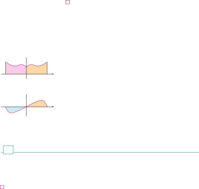
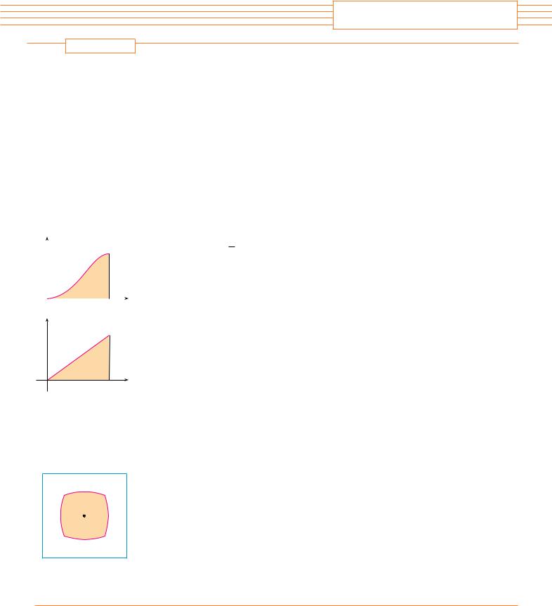
Theorem 7 is illustrated by Figure 4. For the case where f is positive and even, part (a) says that the area under y ! f "x# from !a to a is twice the area from 0 to a because of symmetry. Recall that an integral xab f "x# dx can be expressed as the area above the x-axis and below y ! f "x# minus the area below the axis and above the curve. Thus part (b) says the integral is 0 because the areas cancel.

EXAMPLE 10	Since f "x# ! x6 " 1 satisﬁes f "!x# ! f "x#, it is even and so
	y!22 "x6 " 1# dx ! 2 y02 "x6 " 1# dx
	! 2[71 x7 " x]02 ! 2(1287 " 2) ! 2847			M
EXAMPLE 11	Since f "x# ! "tan x#!"1 " x2 " x4 # satisﬁes f "!x# ! !f "x#, it is odd
and so
	1 tan x
	y!1		dx ! 0	M
	y!1	1 " x2 " x4	dx ! 0	M

5.5E X E R C I S E S

1–6 Evaluate the integral by making the given substitution.


1.	ye!x dx, u ! !x
2.	yx3"2 " x4#5 dx, u ! 2 " x4
3.	yx2 s				dx, u ! x3 " 1
			x3 " 1
4. y		dt		, u ! 1 ! 6t
		"1 ! 6t#4
5.	ycos3% sin % d%,					u ! cos %
6.	y sec2x"21!x# dx,					u ! 1!x

7– 46 Evaluate the indeﬁnite integral.

y x sin" x2# dx

yx2"x3 " 5#9 dx

y"3x ! 2#20 dx

10.

y"3t " 2#2.4 dt

11.

y"x " 1#s

12.

2x " x2

"x2 "

1#2

14.

yex sin"ex# dx

13.

5 ! 3x

15.

ysin &t dt

16.

x2 "

a " bx2

ysec 2%

tan 2% d%

17.

18.

3ax " bx3

ln x 2

20.

a 0

19.

ax b

cos s

22.

sin 1 x 3 2 dx

21.

23.

ycos sin

24.

y 1 tan

sec

ye x s

26.

yecos t sin t dt

25.

1 e x

27.

28.

tan 1x

1 x 2

1 z3

29.

yetan x sec2x dx

30.

sin ln x

cos x

31.

32.

sin2x

e x 1

cos x

33.

yscot x csc2x dx

34.

x 2

35.

sin 2x

36.

sin x

1 cos2x

37.

ycot x dx

38.

cos2 ts

1 tan t

39.

ysec3x tan x dx

40.

ysin t sec2 cos t dt

41.

42.

sin 1x

1 x 4

1 x 2

1 x

x 2

43.

44.

1 x 2

1 x

45.

46.

x 3sx 2 1 dx

sx 2

;47–50 Evaluate the indeﬁnite integral. Illustrate and check that your answer is reasonable by graphing both the function and its antiderivative (take C 0).

47.	yx x 2 1 3 dx							48.	y	sin sx				dx
										s
										s			x
49.	ysin3x cos x dx							50.	ytan2 sec2 d

51–70 Evaluate the deﬁnite integral.
	2								7
51.	y0	x		1 25 dx				52.	y0		s4 3x dx
	1								s
	1		2		3	5			s						2
53.	y0	x		1 2x			dx	54.	y0			x cos x				dx

SECTION 5.5

THE SUBSTITUTION RULE

|||| 407

1 2

t 4 dt

y1 6

55.

sec

56.

csc

t cot

t dt

57.

y 6 tan

58.

1 x

sin x

59.

60.

y 2

x 2

1 x6

61.

62.

cos x sin sin x dx

1 2x 2

63.

x sx 2 a 2 dx a

64.

x sa 2 x2 dx

65.

x sx 1 dx

66.

1 2x

1 2

sin 1x

67.

68.

x s

ln x

1 x 2

1 e z 1

T 2

69.

70.

sin 2 t T

e z

;71–72 Use a graph to give a rough estimate of the area of the region that lies under the given curve. Then ﬁnd the exact area.

71.y s2x 1, 0 x 1

72. y 2 sin x sin 2x, 0 x

73.Evaluate x22 x 3 s4 x2 dx by writing it as a sum of two integrals and interpreting one of those integrals in terms of an area.

74.Evaluate x01 x s1 x4 dx by making a substitution and interpreting the resulting integral in terms of an area.

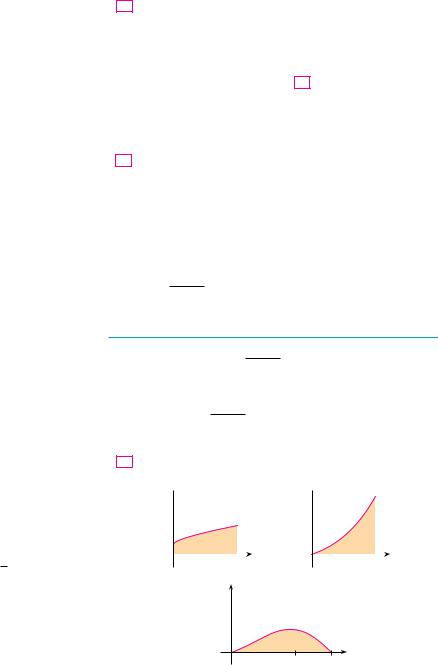
75.Which of the following areas are equal? Why?

y y

			y=2x´
	y=eœ„x
	y=eœ„x

0	1 x	0	1 x
	y

y=esin x sin 2x

0	1	π	x
		2

76. A model for the basal metabolism rate, in kcal h, of a young man is R t 85 0.18 cos t 12 , where t is the time in hours measured from 5:00 AM. What is the total basal metabolism of this man, x024 R t dt, over a 24-hour time period?

408 |||| CHAPTER 5 INTEGRALS

77.An oil storage tank ruptures at time t ! 0 and oil leaks from the tank at a rate of r"t# ! 100e!0.01t liters per minute. How much oil leaks out during the ﬁrst hour?

78.A bacteria population starts with 400 bacteria and grows at a rate of r"t# ! "450.268#e1.12567t bacteria per hour. How many bacteria will there be after three hours?

79.Breathing is cyclic and a full respiratory cycle from the beginning of inhalation to the end of exhalation takes about 5 s. The maximum rate of air ﬂow into the lungs is about 0.5 L!s.

This explains, in part, why the function f "t# ! 12 sin"2&t!5# has often been used to model the rate of air ﬂow into the lungs. Use this model to ﬁnd the volume of inhaled air in the lungs at time t.

80. Alabama Instruments Company has set up a production line to manufacture a new calculator. The rate of production of these calculators after t weeks is

dx	! 5000'1 !	100	( calculators!week
dt		"t " 10#2

(Notice that production approaches 5000 per week as time goes on, but the initial production is lower because of the workers’ unfamiliarity with the new techniques.) Find the number of calculators produced from the beginning of the third week to the end of the fourth week.

81. If f is continuous and y04 f "x# dx ! 10, ﬁnd y02 f "2x# dx.

82. If f is continuous and y09 f "x# dx ! 4, ﬁnd y03 xf "x2 # dx.

5 R E V I E W

C O N C E P T C H E C K

1. (a) Write an expression for a Riemann sum of a function f. Explain the meaning of the notation that you use.

(b) If f "x# ) 0, what is the geometric interpretation of a Riemann sum? Illustrate with a diagram.

(c) If f "x# takes on both positive and negative values, what is the geometric interpretation of a Riemann sum? Illustrate with a diagram.

2. (a) Write the deﬁnition of the deﬁnite integral of a function from a to b.

(b) What is the geometric interpretation of xab f "x# dx if f "x# ) 0?

(c) What is the geometric interpretation of xab f "x# dx if f "x# takes on both positive and negative values? Illustrate with a diagram.

3. State both parts of the Fundamental Theorem of Calculus. 4. (a) State the Net Change Theorem.

83. If f is continuous on !, prove that

yab f "!x# dx ! y!!ba f "x# dx

For the case where f "x# ) 0 and 0 * a * b, draw a diagram to interpret this equation geometrically as an equality of areas.

84. If f is continuous on !, prove that

yab f "x " c# dx ! yab""cc f "x# dx

For the case where f "x# ) 0, draw a diagram to interpret this equation geometrically as an equality of areas.

85. If a and b are positive numbers, show that

y01 xa"1 ! x#b dx ! y01 xb"1 ! x#a dx

86.	If f is continuous on $0,	&%, use the substitution u ! & ! x to
	show that
	&		&	&
	y0 xf "sin x# dx !			y0 f "sin x# dx
	y0 xf "sin x# dx !		2	y0 f "sin x# dx
87.	Use Exercise 86 to evaluate the integral
	&	x sin x
	y0				dx
	y0	1 " cos2x			dx
88.	(a) If f is continuous, prove that			!2 f "sin x# dx
	y0 !2 f "cos x# dx ! y0			!2 f "sin x# dx
	&		&
		&		&
	(b) Use part (a) to evaluate x0 !2		cos2x dx and x0			!2 sin2x dx.

(b) If r"t# is the rate at which water ﬂows into a reservoir, what

does xtt2 r"t# dt represent?

5. Suppose a particle moves back and forth along a straight line with velocity v"t#, measured in feet per second, and acceleration a"t#.

(a) What is the meaning of x60120 v"t# dt?

(b) What is the meaning of x60120 * v"t# * dt?

6. (a) Explain the meaning of the indeﬁnite integral xf "x# dx.

(b) What is the connection between the deﬁnite integral xab f "x# dx and the indeﬁnite integral xf "x# dx?

7. Explain exactly what is meant by the statement that “differentiation and integration are inverse processes.”

8. State the Substitution Rule. In practice, how do you use it?

CHAPTER 5 REVIEW |||| 409

T R U E - F A L S E Q U I Z

Determine whether the statement is true or false. If it is true, explain why.

If f and t are continuous and f "x# ) t"x# for a ' x ' b, then

If it is false, explain why or give an example that disproves the statement.

yab f "x# dx ) yab t"x# dx

If f and

are continuous on

a, b , then

yab $ f "x# " t"x#% dx ! yab f "x# dx " yab t"x# dx

If f and t are differentiable and f "x# ) t"x# for a * x * b,

then f #"x# ) t#"x# for a * x * b.

If f and t are continuous on $a, b%, then

y!11 'x5 ! 6x9 "

sin x

(dx ! 0

yab $ f "x#t"x#% dx ! 'yab f "x# dx('yab t"x# dx(

"1 " x4 #2

If f is continuous on $a, b%, then

10.

y!5

"ax2 " bx

" c# dx ! 2 y0 "ax2 " c# dx

ya 5f "x# dx ! 5 ya

f "x# dx

11.

dx ! !

If f is continuous on $a, b%, then

12.

x02 "x ! x3# dx represents the area under the curve y ! x ! x3

yab xf "x# dx ! x yab f "x# dx

from 0 to 2.

13.

All continuous functions have derivatives.

If f is continuous on $a, b% and f "x# ) 0, then

14.

All continuous functions have antiderivatives.

15.

If f is continuous on $a, b%, then

b s

dx !

b f "x# dx

f "x#

'yab

f "x# dx( ! f "x#

If f # is continuous on $1, 3%, then y13 f #"v# dv ! f "3# ! f "1#.

E X E R C I S E S

Use the given graph of f

to ﬁnd the Riemann sum with six

(b) Use the deﬁnition of a deﬁnite integral (with right end-

subintervals. Take the sample points to be (a) left endpoints and

points) to calculate the value of the integral

(b) midpoints. In each case draw a diagram and explain what

the Riemann sum represents.

"x ! x# dx

y
2		y=Ä
2
0	2	6	x

2. (a) Evaluate the Riemann sum for

f "x# ! x2 ! x 0 ' x ' 2

with four subintervals, taking the sample points to be right endpoints. Explain, with the aid of a diagram, what the Riemann sum represents.

(c)Use the Fundamental Theorem to check your answer to part (b).

(d)Draw a diagram to explain the geometric meaning of the integral in part (b).

3.Evaluate

y01 (x " s1 ! x2 ) dx

by interpreting it in terms of areas.

4. Express

n
lim	sin xi ,x
n l+ i,!1
as a deﬁnite integral on the interval $0,		&% and then evaluate
the integral.

410		\|\|\|\| CHAPTER 5 INTEGRALS
5.		If x06 f "x# dx ! 10 and x04 f "x# dx ! 7, ﬁnd x46 f "x# dx.
	6.	(a) Write x15 "x " 2x5 # dx as a limit of Riemann sums,
CAS

		taking the sample points to be right endpoints. Use a

computer algebra system to evaluate the sum and to compute the limit.

(b)Use the Fundamental Theorem to check your answer to part (a).

7.The following ﬁgure shows the graphs of f, f #, and

x0x f "t# dt. Identify each graph, and explain your choices.

y	b
	b
	c
	x
	a

8. Evaluate:

(a)	y01	d	"earctan x# dx	(b)	d	y01 earctan x dx
		dx			dx
(c)	d	y0x	earctan t dt
	dx

9–38 Evaluate the integral, if it exists.

y12

"8x3 " 3x2 # dx

10.

y0T "x4 ! 8x " 7# dx

11.

y01

"1 ! x9 # dx

12.

y01

"1 ! x#9 dx

! 2u2

13.

14.

(su " 1#

15.

y01

y" y2 " 1#5 dy

16.

y02

y2s

1 " y3

17.

y15

18.

y01

sin"3&t# dt

"t !

4#2

19.

y01

v2 cos"v3# dv

20.

y!11

sin x

1 " x2

&!4

t4 tan t

21.

y!&!4

22.

2 " cos t

1 " e2x

23.

1 !

(2 dx

24.

y110

x2 !

25.

x " 2

26.

csc2x

1 " cot x

x2 " 4x

27.

ysin

&t cos

&t dt

28.

ysin x cos"cos x# dx

29.

esx

30.

y cos"xln x# dx

31.

ytan x ln"cos x# dx

32.

1 !

33.

34.

ysinh"1 " 4x# dx

1 " x4

sec % tan %

35.

36.

"1 " tan t#3 sec2t dt

1 " sec %

37.

y03 * x2 ! 4 * dx

38.

y04 * s

! 1 * dx

;39– 40 Evaluate the indeﬁnite integral. Illustrate and check that your answer is reasonable by graphing both the function and its antiderivative (take C ! 0).

cos x

39.

40.

1 " sin x

x2 " 1

;41.

Use a graph to give a rough estimate of the area of the region

that lies under the curve y ! xsx , 0 ' x ' 4 . Then ﬁnd the

exact area.

;

42.

Graph the function f "x# ! cos2x sin3x and use the graph to

guess the value of the integral x02

"x# dx. Then evaluate the

integral to conﬁrm your guess.

43– 48 Find the derivative of the function.

43.

F"x# ! y0x

44.

F"x# ! yx1 s

t " sin t

1 "

sin x

1 ! t2

45.

t"x# ! y0

cos"t2# dt

46.

t"x# ! y1

1 " t4

47.

y ! ysx

48.

y ! y23xx"1 sin"t4 # dt

49–50 Use Property 8 of integrals to estimate the value of the integral.

49. y13 s		dx	50. y35	1		dx
	x2 " 3
				x "	1

51–54 Use the properties of integrals to verify the inequality.

	1		2		1		&!2 sin x		s	2
51.	y0	x		cos x dx '		52.	y&!4 x	dx '
51.	y0	x		cos x dx '	3	52.	y&!4 x	dx '	2
53.	y01	ex cos x dx ' e ! 1				54.	y01 x sin!1x dx ' &!4

55.Use the Midpoint Rule with n ! 6 to approximate x03 sin"x3# dx.

56.A particle moves along a line with velocity function v"t# ! t2 ! t, where v is measured in meters per second.

Find (a) the displacement and (b) the distance traveled by the particle during the time interval $0, 5%.

57.Let r"t# be the rate at which the world’s oil is consumed, where t is measured in years starting at t ! 0 on January 1,

2000, and r"t# is measured in barrels per year. What does x08 r"t# dt represent?

58.A radar gun was used to record the speed of a runner at the

times given in the table. Use the Midpoint Rule to estimate the distance the runner covered during those 5 seconds.

t (s)	v (m!s)	t (s)	v (m!s)

0	0	3.0	10.51
0.5	4.67	3.5	10.67
1.0	7.34	4.0	10.76
1.5	8.86	4.5	10.81
2.0	9.73	5.0	10.81
2.5	10.22

59.A population of honeybees increased at a rate of r"t# bees per week, where the graph of r is as shown. Use the Midpoint Rule with six subintervals to estimate the increase in the bee population during the ﬁrst 24 weeks.

12000

8000

4000

0	4	8	12	16	20	24	t
						(weeks)

60.	Let
		!x ! 1		if !3 ' x ' 0
		f "x# ! -!s		if 0 ' x ' 1
		f "x# ! -!s	1 ! x2	if 0 ' x ' 1
	Evaluate x!1 3 f "x# dx by interpreting the integral as a
	difference of areas.
61.	If f is continuous and x02 f "x# dx ! 6, evaluate
	&!2	f "2 sin %# cos % d%.
	x0	f "2 sin %# cos % d%.
62.	The Fresnel function S"x# ! x0x sin(21&t2) dt was introduced
	in Section 5.3. Fresnel also used the function

C"x# ! y0x cos(12&t2) dt

in his theory of the diffraction of light waves.

(a) On what intervals is C increasing?

	CHAPTER 5 REVIEW \|\|\|\| 411
	(b) On what intervals is C concave upward?
	(c) Use a graph to solve the following equation correct to two
CAS
	decimal places:
	y0x cos(21&t2) dt ! 0.7
	(d) Plot the graphs of C and S on the same screen. How are
CAS	(d) Plot the graphs of C and S on the same screen. How are
	these graphs related?

;63. Estimate the value of the number c such that the area under the curve y ! sinh cx between x ! 0 and x ! 1 is equal to 1.

64.Suppose that the temperature in a long, thin rod placed along the x-axis is initially C!"2a# if * x * ' a and 0 if * x * $ a. It can be shown that if the heat diffusivity of the rod is k, then the temperature of the rod at the point x at time t is

		C	a	2
T"x, t# !			y0	e!" x!u# !"4kt# du
	a
		4&kt
	s

To ﬁnd the temperature distribution that results from an initial hot spot concentrated at the origin, we need to compute

lim T"x, t#

a l0

Use l’Hospital’s Rule to ﬁnd this limit.

65. If f is a continuous function such that

y0x f "t# dt ! xe2x " y0x e!tf "t# dt

for all x, ﬁnd an explicit formula for f "x#.

66.Suppose h is a function such that h"1# ! !2, h#"1# ! 2,

h."1# ! 3, h"2# ! 6, h#"2# ! 5, h."2# ! 13, and h. is continuous everywhere. Evaluate x12 h."u# du.

67.If f # is continuous on $a, b%, show that

2yab f "x# f #"x# dx ! $ f "b#%2 ! $ f "a#%2

68.Find hliml0 1h y22"h s1 " t3 dt.

69.If f is continuous on $0, 1%, prove that

				y01 f "x# dx ! y01 f "1 ! x# dx
70.	Evaluate		)'n	(		'n	( 'n			(			'n		(	&
	n l+ n		)'n	(		'n	( 'n			(			'n		(	&
	lim	1	1		9	2	9		3		9			n	9
	lim				"			"				" - - - "
71.	Suppose f is continuous, f "0# ! 0, f "1# ! 1, f #"x# $ 0, and
	x01 f "x# dx ! 31. Find the value of the integral x01 f !1" y# dy.

P R O B L E M S P L U S

N The principles of problem solving are discussed on page 76.

N Another approach is to use l’Hospital’s Rule.

Before you look at the solution of the following example, cover it up and ﬁrst try to solve the problem yourself.

EXAMPLE 1 Evaluate lim		x	x sin t	dt .
	'x ! 3		y3 t
x l3				(

SOLUTION Let’s start by having a preliminary look at the ingredients of the function. What happens to the ﬁrst factor, x!"x ! 3#, when x approaches 3? The numerator approaches 3 and the denominator approaches 0, so we have

x	l + as x l 3"	and	x	l !+ as x l 3!
x ! 3			x ! 3

The second factor approaches x33 "sin t#!t dt, which is 0. It’s not clear what happens to the function as a whole. (One factor is becoming large while the other is becoming small.) So how do we proceed?

One of the principles of problem solving is recognizing something familiar. Is there a part of the function that reminds us of something we’ve seen before? Well, the integral

y3x sint t dt

has x as its upper limit of integration and that type of integral occurs in Part 1 of the Fundamental Theorem of Calculus:

dxd yax f "t# dt ! f "x#

This suggests that differentiation might be involved.

Once we start thinking about differentiation, the denominator "x ! 3# reminds us of something else that should be familiar: One of the forms of the deﬁnition of the derivative in Chapter 2 is

F#"a# ! lim F"x# ! F"a#

x la x ! a

and with a ! 3 this becomes

F#"3# ! lim F"x# ! F"3#

x l3 x ! 3

So what is the function F in our situation? Notice that if we deﬁne

F"x# ! y3x sint t dt

then F"3# ! 0. What about the factor x in the numerator? That’s just a red herring, so let’s factor it out and put together the calculation:

lim		x	x sin t	dt		! lim x ! lim		y3x sint	t dt
lim	'x ! 3		y3 t	dt	(	! lim x ! lim		x !	3
x l3	'x ! 3		y3 t		(	x l3	x l3	x !	3
						! 3 lim	F"x# ! F"3#
						! 3 lim	x ! 3
						x l3	x ! 3
						! 3F#"3# ! 3		sin 3		(FTC1)
								3
						! sin 3					M

412

PROBLEMS

y	P{t,!sin(t@)}
y

	y=sin{≈}
	A(t)

O	t	x
y	P{t,!sin(t@)}
	P{t,!sin(t@)}

B(t)

Ot x

FIGURE FOR PROBLEM 8

FIGURE FOR PROBLEM 16

P R O B L E M S P L U S

1.If x sin &x ! y0x2 f "t# dt, where f is a continuous function, ﬁnd f "4#.

2.Find the minimum value of the area of the region under the curve y ! x " 1!x from x ! a to x ! a " 1.5, for all a $ 0.

3.If f is a differentiable function such that f "x# is never 0 and x0x f "t# dt ! $ f "x#%2 for all x, ﬁnd f.

; 4. (a) Graph several members of the family of functions f "x# ! "2cx ! x2 #!c3 for c $ 0 and look at the regions enclosed by these curves and the x-axis. Make a conjecture about how the areas of these regions are related.

(b)Prove your conjecture in part (a).

(c)Take another look at the graphs in part (a) and use them to sketch the curve traced out by the vertices (highest points) of the family of functions. Can you guess what kind of curve this is?

(d)Find an equation of the curve you sketched in part (c).

5. If f "x# ! y0t" x#			1	dt , where t"x# ! y0cos x $1 " sin"t2 #% dt, ﬁnd f #"&!2#.
	s
		1	" t3

6.If f "x# ! x0x x2 sin"t2 # dt, ﬁnd f #"x#.

7.Evaluate xliml0 1x y0x "1 ! tan 2t#1! t dt.

8.The ﬁgure shows two regions in the ﬁrst quadrant: A"t# is the area under the curve y ! sin"x2 #

from 0 to t, and B"t# is the area of the triangle with vertices O, P, and "t, 0#. Find lim A"t#!B"t#.

t l0"

9. Find the interval $a, b% for which the value of the integral xab "2 " x ! x2 # dx is a maximum.

10000

10.

Use an integral to estimate the sum

, s

i!1

11.

(a)

Evaluate x0n .x/ dx, where n is a positive integer.

(b)

Evaluate xab .x/ dx, where a and b are real numbers with 0 ' a * b.

sin t

12.

Find

y0 'y1 s

1 " u4

du dt.

dx2

(

13.

Suppose the coefﬁcients of the cubic polynomial P"x# ! a " bx " cx2 " dx3 satisfy the equation

a "

! 0

Show that the equation P"x# ! 0 has a root between 0 and 1. Can you generalize this result for an

nth-degree polynomial?

14.

A circular disk of radius r is used in an evaporator and is rotated in a vertical plane. If it is to be

partially submerged in the liquid so as to maximize the exposed wetted area of the disk, show that

the center of the disk should be positioned at a height r! 1 " &2

above the surface of the liquid.

15.

Prove that if f is continuous, then y0x f "u#"x ! u# du ! y0x 'y0u f "t# dt(du.

16.

The ﬁgure shows a region consisting of all points inside a square that are closer to the center than

to the sides of the square. Find the area of the region.

17.

Evaluate lim

" - - - "

n l+

'sn sn " 1

sn sn " 2

sn sn " n

(

18.For any number c, we let fc"x# be the smaller of the two numbers "x ! c#2 and "x ! c ! 2#2. Then we deﬁne t"c# ! x01 fc"x# dx. Find the maximum and minimum values of t"c# if !2 ' c ' 2.

413

APPLICATIONS OF

INTEGRATION

The volume of a sphere is

the limit of sums of volumes

of approximating cylinders.

In this chapter we explore some of the applications of the deﬁnite integral by using it to compute areas between curves, volumes of solids, and the work done by a varying force. The common theme is the following general method, which is similar to the one we used to ﬁnd areas under curves: We break up a quantity Q into a large number of small parts. We next approximate each small part by a quantity of the form f x*i x and thus approximate Q by a Riemann sum. Then we take the limit and express Q as an integral. Finally we evaluate the integral using the Fundamental Theorem of Calculus or the Midpoint Rule.

414

<<< < Предыдущая 27 28 29 30 31 32 33 34 35 36 37 3839 / 9139 40 41 42 43 44 45 46 47 48 49 50 51 > Следующая >>>

Соседние файлы в предмете [НЕСОРТИРОВАННОЕ]

#
05.02.202055.36 Mб21Calculus, 7th Edition ( PDFDrive.com ).pdf
#
30.12.201945.82 Mб43Complete Solutions Manual for_ SINGLE VARIABLE CALCULUS Early Transcendentals 7th Edition by Stewart ( PDFDrive.com ).pdf
#
30.12.201918.09 Mб38[James_Stewart]_Single_Variable_Calculus_Early_Tr(BookFi).pdf