Is usually called the r-th moment of the pdf (random variable); more precisely; the r-th moment of the pdf about zero. On the other hand, the r-th central moment of the pdf is given by:

m' = / (x-y) ф (x) dx .

(3.25)

By inspecting the above expressions for m^ and along with equations (3.20) and (3.22), we can see that:

у = m^ (3.26a)

and a² = = ш₂ - y² = m₂ - m²- . (3.26b)

Compare the above result (3.26 a, b) with the analogy to mechanics men­tioned in sections 3.1.3 and 3.1.4.

3.2.4 Basic Postulate (Hypothesis) of Statistics, Testing

The basic postulate of statistics is that "any random sample has got a parent random variable". This parent random variable xtR is usually called population and is considered to be infinite. It is common in stat­istics to postulate the pdf of the population for any random sample, and call it the postulated, or the underlying pdf. Such a postulate may be hence tested for statistical validity.

In order to be able to test the statistical validity we have to assume that the sample can be regarded as having been picked out, or drawn from the population, each element of the sample independently from the rest. This additional property of a sample is required by the standard definition of a random sample as used in statistical literature. However, since the present Introduction does not deal with statistical testing we shall keep using our original, more general definition.

There are infinitely many families of PDF¹s• Every such family is defined by one or more independent parameters, whose values characterize the shape of its pdf. The individual members of a family vary according to the value of these parameters. It is common to use if possible, the mean and the standard deviation as the pdf¹s parameters. The less parameters the family of pdf¹s contains the better; the easier it is to work with.

The usual technique is that we first select the "appropriate" family of pdf¹s on the basis of experience and then try to find such values

of its parameters that would fit the actual random sample the best. In other words, the shape of the postulated ф(х) is chosen first; then, its parameters are computed using some of the known techniques.

Since we shall be dealing with the samples and the random var-

iables (populations) at the same time, we shall use, throughout these notes, the latin letters for the sample characteristics, and the corresponding greek letters for the population characteristics as we have done so far.

3.2.5 Two Examples of a Random Variable

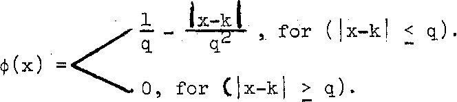
Example 3.17: As the first example, let us investigate a random variable x

with rectangular (uniform) PDF which is symmetrical

around a-value .x;= k. *-:E^:it" the -probability

of x < k-q and x > k+q, be zero. Obviously, this PDF has the

following analytical form (see Figure 3.13):

,h, for (k - q < x < к + q)

0, for (x < к - q) and (x > к + q).

This can be written in an abbreviated form as:

<h, for (j.x-k|. < q). v 0, for (]jc - k| > q).

The above ф contains apparently three parameters k, q and h.

However _э only two are independent, since one can be eliminated

from the condition (3*15)> i.e.:

/ ф(x) dx = 1

—00

that must be satisfied for any ф to be a PDF. Let us

eliminate for instance the parameter h. We can write: oo k-q k+q

/ ф (x) dx = / ф (x) dx + / ф (x) dx + -«о »oo k-q

00

/ ф (x) dx k+q

k+q

= 0 + / hdx + 0

k-q

= h / dx = h [x], = 2hq. = 1. . к—q

k-q ^u

This means that h _э and therefore:

2q

<l/(2q), for (|.x - k| < q) 0₉ for (|x - k| > q)

T he corresponding CDF to the above ф is:

0, for (x< k-q)

^X 1 ^x 1

¥(x) = / ф(х) dx =f~— — / dx. = — (x-k+q), for

^ k-q

—.00

(|x - fr| < q).

1, for (x > к + q) ₇

and is shown in Figure 3.1*+.

From the above figure we see that the functionфis linear in the interval over which ф / 0, and is constant everywhere else. Note

dx

The mean of the given PDF is computed from equation (3.20) as follows:

\i = f хф (x)dx

J" xc k-q

k+q 2 k+q

2q 2 ^Jk-q

2q

¹ ' .dx = 7Г

= (k² + 2kq + q² - k² + 2kq - q²)

This result satisfies our expectation for a symmetrical function

around k. The variance of the given PDF can be obtained from

equation (3.22), yielding

2 _ _r°° p _л k+q

a (х-цГ ф(х) dx = ^ / (х-кГ dx =

1 ,^k+<1 2_a 2k ^ _A к² ,^к+1 _л k~q ^ k-q ⁴ k-q

= T- tl-J, - ^{2k + k}

2q 3 k-q

= ^ (k³ + 3k²q + 3kq² + q³ - k³ + 3k²q - 3kq² + q³) - k²

6k q ^ 2al , 2 q~

6q 6q 3

1 1

Since к = у and q = /За, then h = — - 7777-, and we can

2q 2/3a

express the given rectangular PDF, which we will denote by R, in terms of its mean у and its standard deviation о as follows:

for (-|x-ji|) < /За)

R(-y, а ; x) = ф(х) ==<^

V.O, for ( |x - ji| ) > /За) _#

Similarly, we can express its corresponding CDF, which we will

denote by R^, in terms of;ц and а, as follows:

, 0, f©-apvtx^T< у - /За).

R (ji,cr;x) = f(x) =^ ^7^7 (x-y,+/3a), for (|x~y| < /За).

1, for (x > у + /За) , Assume that we would like to compute the probability of x e [ y-а, y.+a], where x has the rectangular PDF . This can be done by using equation (3.l6c) and Figure 3.15 > as follows:

у+а

Р( у-а < х < у +а) = / ф(х) dx

у+а = / у-а

_{г7з5 ta в W [2а3}

The above probability is given by the shaded area in Figure 3.15.

Similarly, for this particular uniform PDF, we find that: P(y-2a < x < у + 2a) = P( y-3a < x < p+ 3a) = 1.0

In"statistical "testing, we :6ften. need to compute the moments of the PDF (see .--secti^H:З.2.3). Let'ua, .-for instance, compute the third moment m^ about zero of the rectangular PDF,.. We will use equation Ov2U') ₉ - i. e."

3 1 .

■Х „ и dx

°° ' у +/3с

ш - / х ф(х) dx - / * ^

-⁰⁰ у-/За

1 х^ ^^За

₌ 27за" ^[Т~^] /, Р -/За

= §73^ (S^ou³ + 2W3 а³_р)

3 2 = у + За у

Example 3.18: As a second example let us investigate a random variable with

a triangular PDF, which is symmetrical around x = k.. Let us

Figure 3«l6

assume that the probability of x < к - q and x > к + q, be zero. We may write (see Figure 3.l6):

Ф(х) =

■6, for (х < к - q).

(х -k + q), for (к - q < х < к).

О, for (х > к + q).

— £«х + к + q) , for (к < х < к + q).

This .can be rewritten in the following abbreviated form as:

7 (q - |x - k|), for (|x - k| < q)

0 , for (|x - кj > q) .

From the above, we can see that the triangular PDF has the same parameters (k, q, h) as the uniform PDF of example 3.17• Let us again eliminate the parameter h from the condition

/ ф(х) dx = 1. This integral is nothing else but the area

.00

of the triangle, so. that we. can write.:.':—'v 2q * h = qh = 1. This^: gives■. us : h = ~₉ and hence,

The computations of the mean and the variance of the triangular PDF can be performed by following the same procedure as we have done for the rectangular PDF in example 3.17. We state here the results without proof, and the verification is left to the student•

The mean у of the given triangular PDF equals to к , and the

2 12

variance a comes out as q .

Since к. = у and q = /ба _э we ean /agaia respites' the tri­angular PDF, which we will denote by T, in terms of its mean у and its standard deviation а, as follows:

1 . Ji^l _э for(|x-ii| < /ба)

T (у_э cr -;x) = ф(х) =/

* 0, for ( |x-y| > /ба). The corresponding CDF is given by: '0, for (x < у - q)

x

Y(x)

y-q. q.

1, for (x > У + q), and is shown in Figure 3.17•

0,0

Д f-*^ /> 1		i ^

Figure 3.17

The integral in the above equation can be rewritten as:

б^

k-q'⁴- i² \ ц

^{/ q + * - и- ах for (х < )}

/ q, + х - у _{dx +} ^Х CL^i.

for (x > у).

and we get:

x 1 1 2 x

—о / (q + x- y)dx = ~ {77 [x ] + (q-y) [x] q^ ^ _n2 2 y-q ^ y-

^ y-q ч

= ~₂ {|"(x²~y²+2iiq~q²) + (q-y) (x-y+q)}

12 2 2

= —— {x -2yx+y +2q(x~y) + q }

2q^

2

- (x-yi) ₊ U-u) 1

20² 4 ² ■

Similarly,

\ f^X (d-x₊u) dx = - ₊

q. U 2q q

and

_л q + x- y„ 1 У-q ⁴

Finally, we can express the CDF , which we are going

to denote by , in terms of the mean у and the >sta1tidard deviation a, as follows:

0, for (х <_ у - /бег)

i-Mll ₊ i*zHi ₊ 1 _{for (у} _ _{/ба }}

12а /ба

Т_с(у, а; х) = Ч»(х) =^

Г ^J2E^~ ⁺ + (u 1 х < у ₊ /ба)

12а

1, for (х > у + /ба)

By following the same procedure as in example 3.17,- we can compute the probabilities: P (y-a <_ x у + a), P (y-2a x <_ у + 2a) and P (у-За _< x <_ у + За) as well as the third moment m^ about zero for the triangular PDF. Again, we give here the results, and the verification is left to the students

P(y-a £ x <_ у + a) = 0.66 ,

P(y-2a £ x <_ у + 2a) = 0.97 ,

P(y-3a < x < p + 3a) =1 and m^ = у³ + За²у .

3.3 Random Multivariate

3.3.1 Multivariate, its PDF and CDF

Analogically to the ideas of stochastic function and stochastic variable given in section 3.2,1, we introduce the concept of a multi­valued stochastic function

Xe {U -> R^S}

in the s-dimensional space.

We note that X is a vector function, i.e. , X(u) can be written

as:

/12 s s

X(u) = (x (u) , x (u) , . .. , x (u) ) e R , u e U.

The individual components x"^ (u) £ R, j = 1, 2, . .. , s are called components or constituents of X(u) • We also note that each component x^ of the stoch­astic function X can be regarded as a random variable (univariate) of its

i i

own. One particular value of x may be denoted by x^*) and similarly a

particular value of X may be denoted by

⁼ ^i^r ' • • •' • Note that a specific value of X is a sequence of real numbers (not a set), or a numerical vector.

The pair (X(u), ф(X)), where

ф(Х) = ф(х\ x², . .., x^S) с {R^S ~* R} (3-27)

s

*The superscripts and subscripts here are found very useful to distinguish

between the components x³, j = 1, 2, ..., s of the multivariate X, and

the elements x*?, l ~ 1, 2, • • • , n * of the univariate (random variable) x^J .

is a non-negative, integrable function on R is called a random multi­variate or simply a multivariate.

We can speak of a probability of X £ [X_q, X^]С R , and define it

as follows:

(3-28)

Here the integral sign stands for the s-dimensional integration; dx for

1 2

an s-dimensional differential, i.e. dX = (dx , dx ,

cbc) and

X = (x¹, x², ... x^S) , X- = (x?*, x², .xf) are assumed to satisfy о о о о 1 11 1 ^л

the following inequalities:

x^J > x^{D X}l - ^Xo ' j = 1, 2,

Note that in order to be able to call the function ф a PDF, the following condition has to be satisfied:

/ ф (X) dX = 1 .

s

R

(3-29)

A complete analogy to the one-dimension 1 or univariate case (section 3.2.2) is the definition of the multivariate CDF. It is defined as follows:

X

¥(X) = / ф(У) dYe {R ■> [0, 1]}

(3-30)

where Y is an s-dimensional dummy variable in the integration.

Example 3.19: Consider the univariate PDF shown in Figure 3.12. This be11-shaped PDF is known as the normal or Gaussian PDF (to be discussed later in more details), and is usually denoted by N,

in terms of its у and a we have

ф(х) = N(y, a; x) .

Then the multivariate normal PDF in two-dimensional space, i.e. 12

ф(Х) = ф(х , x ), would appear as illustrated in Figure 3~l8.

Figure 3-l8.

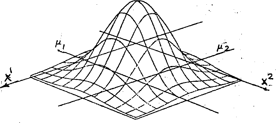
In the two-dimensional space, ф(Х) is called a bivariate PDF,

and the bivariate normal PDF illustrated above can be expressed as

ф(Х) = N(y_x, У₂, а_±9 a₂i X)

1

2

3.3.2 Statistical Dependence and Independence

The PDF, ф, of the multivariate X may have a special form,

namely

s

ф(Х) = ф.(х¹).ф.(х²) ... ф (x^S) = П ф. (x^J) *

^s 5=1 ³

In this case, the integral in equation (3-28) can he rewritten as:

X.. X ^ .

/ ф(Х) dX = /_х .П_ ф. (x^J) dx^J

S X"

= П /

О

(x^J ) dx^:

(3-31)

Remembering that each component x^J of the multivariate X can be regarded

as a univariate, and regarding ф. as the PDFs of the corresponding

J

univariates we can rewrite equation (3-31) as:

s j . s ...

П f^Xl ф . (x^J )dx^J = П P(x^J 1 x^J £ x^ ) • j=l x^ ³ j=l °

Comparing this result with equation (3-28), we get the relationship

between the probabilities

(3-32)

This relation can be read as follows: "The combined probability of all the components satisfying the condition: x^ £ x^J <_ x^, equals to the product of the probabilities for the individual components", and obviously satisfies the definition of the combined probability of

independent events (section 2.3). Hence, the components x of such a multivariate X are called statistically independent. The PDF from example 3.19 is statistically independent.

If the PDF of a multivariate cannot be written as a product of the PDF's of its constituents, then these constituents are known as statistically dependent. In this case, the probability P(X £ X £ X^) is not equal to the product of the individual probabilities.

It can be shown that for statistically independent components

we have

/ ф. (к³) dx^D = 1, j = 1, 2, ..., s.

R 3

3.3.3 Mean and Variance of a Multivariate

The sequence

Г

fl = (u., u_, ... _r u ) = E*(X) e R ,

12 s

(3-33)

where

у. = / x^J ф (X) dX = E* (x^J)e R, j = 1, 2,

3 _Rs

(3-34)

is called the mean of the multivariate X. The argument of the operator E (i.e. the s-dimensional integral) is X. ф (X) = (х\х², . .. ,x^S) *ф (x\x² ,. .. Similarly the variance of the multivariate X is given by

(3-35)

where

a? = / (x^j-y.)² ф(Х) dX 3 _Rs 3

= E* (x^]-]j.)²) £ R, j = 1, 2, . . . , s. (3-36)

Note that we can write again

E*(X-y)² = Е*(Х~Ё*(Х))² = E*(X²) - ]i² , (3-37)

and

E*(x^j-y.)² = E*(x^j-E*(x^j))² = E*((x^j)²) - y^?; .(3-38) 3 3

The variance of the multivariate does not express the statis­tical properties in the multi-dimensional, space as fully as the variance of the univariate does in the one-dimensional space. For this reason, we extend the statistical characteristics of the random multivariate further and introduce the so-called variance-covariance matrix (see section 3.3.4).

Let us now turn our attention to what the mean and the variance of a "statistically independent" multivariate look like. For the stat­istically independent components x³, j = 1, 2, ..., s of a multivariate X, we obtain

-i s о 0

v. = f x^J П ф.(х") dx* ³ r^s n=i *

= / [x³ $.(x³) ( П ф₀ (x^£)dx^X)dx^j] (3-39)

= / x^.(x^j)dx^j • П / ф₀(x^£)dx^Л . ^{R 3} £=1 ^{R 1}

Here, according to section 3.3.2, all the integrals in equation (3-39) after the П-sign are equal to one, and thus we have

Уц = /_DxV (x^j) dx^j, j = 1, 2, s . (3-40)

J ^K D

Similarly,

— 1, 2,

s.

(3-41)

Thus for the statistically independent X, we can compute the mean and

the variance of each component x³ separately , as we have computed

a₀ of the PDF from example 3.19.