Introduction

In technical practice, as well as in all experimental sciences, one is faced with the following problem: evaluate quantitatively para­meters describing properties, features, relations or behaviour of various objects around us. The parameters can be usually evaluated only on the basis of the results of some measurements or observations. We may, for example, be faced with the problem of evaluating the length of a string. This can be measured directly. Here the only parameter we are trying to determine is the observed quantity itself and the problem is fairly simple. More complicated proposal would be, for instance, to determine the coefficient of expansion of a rod. Then the parameter—the coefficient of expansion—cannot be measured directly, as in the previous case, and we have to deduce its value from the results of observations of length, by performing some computations using the mathematical relationship connecting the observed quantities and the wanted parameters. The more complicated the problems get, of course, the more complex is the system whose parameters we are trying to determine. Obviously, the determination of the orbital parameters of a satellite from various angles observed on the surface of the earth would be an example of one such still more sophisticated task.

The adjustment is a discipline that tries to categorise those • problems and attempts to deal with them symmetrically. In order to be able to deal with such problems systematically the adjustment has to use a language suitable for this purpose, the obvious choice being mathematics.

Hence, the problem to be treated has to be first "translated" into the language of mathematics, i.e., the problem has to be first mathematically formulated. The mathematical formulation of the problem would really be the mathematical formulation of the relation between the observed quan­tities (observables) and the wanted quantities (parameters). This relation­ship is called the mathematical model. Denoting the observables by L (L stands for one, two, or n quantities) and the parameters by X (X stands for one, two or m quantities) the most general form of the mathematical model cna be written as

F (X, L) = 0 .

The above equation merely states that there is a (implicit) relation between the observables and the parameters. The formulation of an actual mathematical model has to be done taking into account all the physical and geometrical laws—simply using the accumulated experience. The com­plexity of the mathematical model reflects the complexity of the problem itself. Thus the mathematical model of our first problem is practically trivial:

X = L

where X is the wanted length and L is the observed length.

The mathematical model for the coefficient of expansion a of the rod is more complicated, namely, for instance

1=1 (1 + at) о

where a = X, the observed length % and the observed difference in temper­ature t create L and £ is another parameter (length of the rod at

a fixed temperature) which we happen to know. The mathematical model for the satellite orbital elements would be more complicated still.

Once the mathematical model has been formulated it can become a subject of rigorous mathematical treatment, a subject of adjustment calculus. Hence, the formulation of the mathematical model itself is to be considered as being beyond the scope of adjustment calculus and only the various kinds of mathematical models alone constitute the subject of interest.

There is one particular class of models, that are very often encountered in practice, and that can be termed as overdetermined. By an overdetermined model we understand a model which does not have a unique solution for X because there are "unnecessarily many" observations supplied. This can be the case, say, with our first example, if the length is measured several times. The model in this case would be formulated as

X = A

X - i₂

X - £_n ,

where £ , £«, £ are all encompassed by the symbol L. Or, in the

JL <<£ П

second example, we may have

£ = £ (1 + at.) l о 1

£₀ = £ (1 + at₀) z о *

where (i^, . .., t^, t^, •.., t^) = L.

As we can easily see, these overdetermined models may or may not have a unique solution. They usually have not. Therefore, in order to produce a unique solution of some kine, we have to assume that the observations were not quite correct, that there were errors in their determinations.

This leads us into the area of the theory of errors with its prerequisites—the theory of probability and statistics. With the help of these disciplines we are aboe to define the most probable unique solution (if it exists) for the parameters of the mathematical models. We also are usually able to establish the degree of reliability of the solution.

The notes are divided into six sections: Fundamentals of the intuitive Theory of Sets, Fundamentals of the Mathematical Theory of Probability, Fundamentals of Statistics, Fundamentals of the Theory of Errors, Least-Squares Principle, Fundamentals of the Adjustment Calculus. The first four sections describe the relevant parts of the individual fields that are necessary to understand what adjustment is all about. They, by no means, claim any completeness and it is envisaged that an interested student will supplement his reading from other sources, such as those listed at the end of these notes.

A separate section (5) is devoted to the philosophical basis of the adjustment calculus. Although not very extensive it should be regarded important, giving the reasons why the least-squares technique is used in adjustment.

Finally_f the last section deals with the basics of the adjust­ment proper. Here again, only the introductory parts of the adjustment calculus could be treated with the understanding that only the subsequent courses will develop the full picture.

Throughout the course emphasis is placed on the parallel develop­ment of concepts of "discrete statistics", i.e. statistics of random samples, and "continuous statistics", i.e. statistics of random variables. While random samples are the quantities we deal with in every-day practice, the mathematical tools used are predominently from the continuous domain. Good understanding of the interplay of the two concepts is indispensable for anyone who wants to be able to use the adjustment calculus properly.

The bibliography given at the end of these notes lists some of the useful books dealing with statistics and adjustments. Interested reader is recommended to complement the reading of these notes by turning to at least some of the listed sources.

1.' РШШЖЕЖТАЬЗ OF THE IITUITIVE THEORY OF SETS

' Sets» Elements and Subsets

A set is an ensemble of objects (elements) that can be distin­guished one from another. The set is defined when all its elements are defined.

ГО'- , Q? , U.18 } ,

Example 1.1: A_n =

/1

A, =

A„ =

R

{ 1, 8, 15, d , 0, -Or > h} ₉

{ 0, 1} ,

{all the left feet} _s

{all the cities with more than one million inhabitants in lew Brunswick} ,

{all the real numbers} , and

I e {all the positive integers} , are all sets. The text within the brackets {...} is known as the list of the set. If an element a exists in the list of a set A, ve say that the element a belongs to the set A, and this is denoted by

a e A ,

which is read as ^tTa belongs to A^ft. On the other hand, if an element & does not belong to a set A, we write

a & A j

which is read as "a does not belong to д" •

Example 1.2: Referring to Example 1.1, we see that:

/i * -J

8 e A2 5 ² i A-^ and a right foot i A^<

A part of a set G is called a subset of G whether it contains one or several elements. The fact that a set H is contained in G is hence written as

HC G

If H is not contained in G, i.e. if not all the elements of H are at the same time elements of G₉ we write

H ф G .

Example 1.3: Referring to Example 1.1, we see that:

A₃e ^ ₉ {2 , 35 , 118} О I ,

{1.8 , 3 , 6.2} С R, and {

A set which does not contain any element is known as the empty (void or null) set, and is denoted by 0 .

Example 1.4: The set Ag = {all people taller than 10 feet}

contains no elements, i.e. Ag = 0 • Also from Example 1.1, we find that A_n = 0 . The sets are called equal if they contain the same and none but the same elements.

Example 1.5: All the following sets are equal

{1 ₉ 2 , 3} , {3 , 1 , 2} , {2 , 3 , 1} , ....

1.2. Progression arid Definition Set A progression £ is an ordered (by ordered we mean that £ is arranged such that each of its elements has a specific position) ensemble of objects (elements) that may not all be distinguishable one from another. The definition set D of a progression £ is the set composed from all the distinguishable elements of £. In such a case, we shall also say that D

belongs to £.

Example 1.6: I = -(1 , 2 , б^О^, 2,1,8,0? ) > is a progression, and its definition set D is given by D = {1 , 2 , 8 , Q? } .

At this point, the difference between a progression and a set

should be clear in mind. For instance, the progression

( <£cf* _ь 8 , 2 , 1 , 1 , 2 ^ ^2 1 represents a different progress­ion than the one given in Example 1.6. However, the sets { С^оЛ 8 , ^ , 2 , 1} , {2 , 1 , 8 , dxf^ , C? h ... are all the same as the definition set D in Example 1.6.

1.3. ' Cartesian Product of Sets The Cartesian product of two sets A and В is a set, called the

product set and denoted by A x В (reads A cross B), whose elements are all

the ordered two-tuples of elements of the component sets A and B. Hence,

if a e A and b e B, then the two-tuple (a,b) e A x B. However, if b i A

or _a i B₉ the two tuple (b,a) i A x B.

The above definition can be extended to more than two sets, say

n sets. In such a case, the elements of the product set will be all the

ordered n-tuples of elements of the component sets. Accordingly, we can

define the Cartesian n-power A³¹ lor A^. if no danger of confusion with indexed

set exists} of a set A as the Cartesian, product of the same set A with itself n-times.

Example 1.7: If A = {3 , 1 , 5} and В E {2 , h} , then the product set

A x В is A x В = {(3 ,2), (3 , h)₉ (1 ,2), (l , k), (5 , 2), (5 , h)} . Referring to Example 1.1, we can easily see that: ( rO- , -6': ) e A x A₀ , (U.18 , С ) e A. x A₀ ,

) 'i A_x x A₂ but ( 1 , Z> ) e A₂ x A_x , (1 , 2 , 15 , 1 , 8) _e i⁵ , and (5.l6, 3.26, 1, 0, l) e R

^r"- Intersection of Sets

The intersection of two sets A and B, denoted by А п В, is a set which is a subset of both A and В and does not contain any elements other than the common elements to A and B. The intersection of two sets can be represented by the shaded area in Figure 1.1. Diagrams of this kind are called "Venn diagrams".

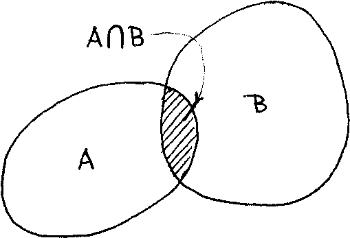
Figure 1.1

From the above diagram we can easily see that

А Л В = В П А . Example 1.8: Referring to Example 1.1, we find that:

а л a = { :o: }, ro i = i ,

А₂П I = {1, k₉ 8, 15} , and А₃П A₂ = {0,1} = A .

Note that we can define a subset A of В as such a set whose intersection with В is A itself. In other words, if AC В then А П В = A, or vice versa (see Figure 1.2).

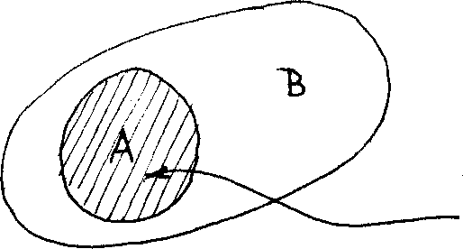
_АГ\В>

Figure 1.2

If ап в = Ф₉ then the sets A and В are said to be disjoint sets. The intersection of n sets A^, Ag, .,. , is usually denoted by

n

П A. . where i=l

n

П A. = А. п А_ЛП A₀ . . .Л A . . ' i 1 2 3 n

i=l

This is illustrated in Figure 1.3 by the common area to all sets.

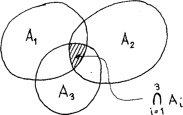
Figure 1.3

1.5 • Union, of Sets

The union of two sets A and B, denoted by AU B, is a set that contains all the elements of A and В and none else. Similar to the inter­section, the union of the two sets is represented by the shaded area in

Figure ±Л

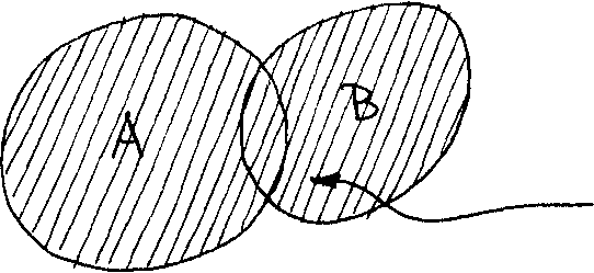
Figure 1Л

The union of n sets A_ , A-. ... , A is denoted Ъу

12 n ¹⁷

n

\J A. , where

i

i=l

\J A. = A U A U A ... UA

_±=1 ± ± г з n

Example 1.9: Referring to Example 1.1, we obtain

U A, M бУ, & , , 1, 8, 15, с ,

i=l ¹

О,Л } ₉

and I u R н R . Thinking of the union as the addition of sets, the subtraction of two sets is known as the complement of one into the other. Referring to Figure 1.5 j and considering the two sets A B, the set of all the elements contained in В and not contained in A is called the complement of A in В_э and is denoted by В - A.

Figure l.g

Example 1,10: Referring to Example 1.1_э we get:

The complement of A~ in A_n Is

j d

^{A0 — Aq = {85 15» с , ;0,: , , and}

R-I ^{ all real numbers that are not integers }.

1.6. Mapping of Sets

f is called a mapping of A into В if it relates one and only one element from В to each element of A. This means that for each element a e A there will be only one corresponding image b e В (see Figure 1.6).

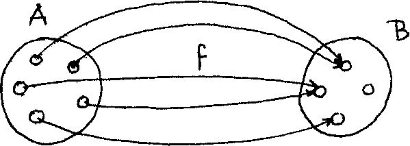
Figure 1.6

Note here that the one-to-one relationship (i.e each b e В has got one

and only one argument, a A), is not required. We shall denote any such mapping

by

f e {A -> В} ,

and read it as "f is an element of the set of all the mappings of A into B",

or simply ^,ff is a mapping of A into в" , or ⁿf maps A into b".

If the elements of В are all images of the elements of A, then f is called an onto mapping, or simply we say that ^,ff maps A onto B".

If A and В are numerical sets, then f is called a function (which gives the mathematical relationship between each a e A and its corresponding image b e B). In this case, the image b of a will be nothing else but the functional value f(a) .

Example 1.11: Given the set A = {a^, a^, a^} = {2, -1, 3} and the mapping

3

f e {A ~* B} , where f(a^) = a.^ for each a. e A, i=l,2,3₅

fhen the images b^ e В are computed as the functional values

3

of the corresponding elements a. e A, i.e. b. * f(a.) = a. ,

^ i l l l

which give Ъ_± = (2)³ =8 , b₂ = (-l)³ = -1, and b_g = (3)³ = 27.

Generally, f is an into function, hence we write

(8, -1, 27) e В . However, if f is an onto function, then

the image set В of this example is given as

В = {8, -1, 27} .

1.7- Exercise 1

1. Which of the following sets are equal?

{t, r\ s}> {s_} r, t} > Cr, s, (t% s, r} .

2. Let A =' {d}, В = {с, d}, С = {a, b, с} , D = {a, b} and H = {a, b, d}; (i) is В С D 1 (ii) is С :- В ?

(iii) is DC С * (iv) is В Ф H ⁷

(v) isA.cH ] (vi) is(AUD)cH ?

(vii) is (апв)<£С ? (viii) is (нп'С) 2 D 2

3. Let U = {1, 2,3, ...,8,9} , a = {l, 2, 3, k} , В = {2, k, 6, 8} ,

С = {3, k, 5, 6} and D =' {1, 3, 5.» 7, 9h then find the following: (i) bud • (ii) аПс <

(iii) A U В ; (iv) U - A ;

(v) a set H, which is a subset of all the sets U, A and D. k. Considering the following Venn diagram with the sets А, В, С, D and H, indicate by shading the suitable areas on separate diagrams, the following sets:

(i) dus )

(ii) HflC ;

(iii) cf)B ;

(iv) A - с ;

(v) В U С j

(vi) (A.- B)U (вПс) j (viii) A - (C U В) •

5. Considering the two sets:

A = {3, h₉ 0, -1} and В в {-2_Э 5) » find the Cartesian products A x В

2

and В x A. Also find the second power В of the set B.

6. Given the set X = {-2, -1, 0, 1, 2} , with f e {X + Y}. If for each x e X, f (x) = x +1, find the image set Y considering that f is an onto function.