In very much the same way as we postulated

l = y_£ and S_L = a_A

for the univariate case as discussed in section U.7. This postulate allows us to work with continuous variables in the mathematical model and write it as:

F(L, X) = 0 (6.5)

understanding tacitly that each value X has- its counterpart L.

From now on, we shall write L for E(L)^and X for the statistical estimate of . X • Hence the mathematical model (6.5) becomes

F(L, X) = 0 , (6.6)

which consists of r functional relationships between L and X.

From the point of view of the mathematical model F(L, X) = 0, the statistical transformation can be either solvable (if s > n) or unsolvable (if s < n), If it is solvable then we may still have two distinctly different cases:

л,

(i) either the model yields only one solution X (when r = s = n) by

using the usual mathematical tools, i.e., X is uniquely derived from L;

(ii) or the mathematical model is оverdetermined (when r, s > n) and cannot be resolved for X at all by using the ordinary mathematical tools, since an infinite number or different solutions for X can be found.

The first case we have met in example (6.1) where the determina­tion of X from L does not present any problem from the statistical point of

view. The only problem is to obtain E from L and E . This problem, known

X L

as propagation of errors, will be the topic of the next section.

If the model is overdetermined, or as we often say, if there are redundancies, (redundant or surplus observations) then the problem of trans­forming (L, E ) -> (X, E ) constitutes the proper problem of adjustment.*)

L X

6.3 Propagation of Errors

6.3.1 Propagation of Variance-Covariance Matrix, Covariance Law

The relationship between e and e for a mathematical model

XL

F(L, X) = 0

is known as the propagation of variance-covariance matrix. Such relationship can be deduced explicitly only for explicit relations

X = F(L) .

To make things easier, let us deduce it first for one particular explicit

Л mm

relation, namely the linear relation between X, and L, i.e.

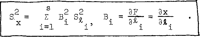
* It has to be mentioned here that in practice we are in both cases working with E- and E£, the variance-covariance matrices of L and X rather than E^, E^ belonging to the samples L and X. The expressions for E-, E^ are derived in 6.4.4.

X = В L + С

where В is indeed an nby s matrix composed of known elements *). Note that X is determined uniquely, as required. We want to establish the transition

Z = e((l-l) (l-l) ) -> E where L = e(l).

(6.8)

We can write:

Z_x = E((X-E(X)) (X-E(x))¹). (6.9)

Here X = BL, and according to the postulate introduced in section 6.2 we can write:

Hence

e(b l+ c) = в e	(l)	+ с = в £ + с.
Ev = e ((bl -	bl)	(bl - bl)t)
= e (b(l -	l)	(b(l - l))t;
= e (b(l -	l)	(l - l)t bt)
= be ((l -	l)	(l - l)t) bt =

Е„ - Б L В

X 1j

(6.10)

*j This matrix b, which determines the linear relationship between x and

L is sometimes called the "design matrix","the matrix of the coefficients" of the constituents of L in the linearized model, or simply the "coef­ficients matrix".

This formula (6.10) is known as the law of propagation of variance covariance¹ matrix, or simply the covariance law.

Example 6.2: Assume that the variance-covariance matrix of a given

multisample L = Л^» £ ) was found to be

^ZL ⁼

2. 0

3. 1 1 k J

If a multisample X = (x^, x^) is to be derived from L according to the following relationships:

"^"1 ~~ ^1 "" ~* ^З^э

^2 " 2Z^ + ^2 »

determine the variance-covariance matrix of X.

It can be seen that the above relationships between the components of X and L are linear, and our mathematical model can be expressed as:

i.e.	X =	В L
	2,1	2,3 3,1
"xl		Г 4 10-3
		2 10
, 2		j

2'

This indicates that the coefficients matrix В is given by:

7

0

В =

i Uo

The variance-covariance matrix l of X is given by equation (6.10) i.e. , in our case:

3	2	0
2	3	1
0	1	1+

= В

t

2,2

0 1

h ^B

2,3 3,3 3,2

■3.

0

1

0 -3

3 -1

8 7

-12 1

39 5

5 23

i.e.

39 5 5 23

Now we shall show that the propagation of variance-covariance matrix can be deduced even for a more general case, namely the non-linear relation between X and L, i.e.

X = F (L) (6.11)

when F is a function with at least the first order derivative. Here we

have to adopt another approximation yet. We have to linearize the relation (6.11) using, for instance, Taylor^f s series expansion around an approximate ■ value L° for L .

X = F(L°) ₊ ^

(L - L ) + higher order terms,

where

dL 'L = L

Ikl

Taking the first two terms only, which is permissible when the values of

the elements in ZL are much smaller than the values of I., we can write:

L l

_{X - F(L°) + B(L » L°) (6.12)}

Эх.

derivatives -гт~~ J

where В is again annby s matrix but this time composed from all the partial

*). Applying the expectation operator we obtain

realizing that E(F(L⁰)) = F(L°) and E(L°) = L° (because L° is a selected vector of constant values) :

E (X) = E (F(L°) + B(L - L°))

= F(L°) + B(E(L) - L°). (6.13)

Subtracting (6.13) from (6.12) we get:

X - E (X) = B(L - E(L)) = B(L - L) (6.lk)

and we end up again with

E_x = BE_LB^T , (6.15)

realizing that £_x_g(_x) = ^_x •

X =

* Explicitly, if we have

4		xl		. . , it ) s
		X2	(* ^29 *	• • > V
X . n		X n	( ^-^5 ^25 *

:.-:^h'em:^:.the matrix В will take the form:

	3xi	ЭХ1
Э£1		s
ЪХ2
Ы	Э£2 '	s

Э£_

Эх г

Э£„

Эх п

Э£

1U2

Hence the linear case may he regarded as one particular instance(special case) of the more general explicit relation, yielding therefore the same law for the propagation of variance-covariance matrix, i.e., the same covariance law. It should he noted that the physical units of the individual elements of both matrices В and £^ must he considered and selected in such a way to give the required units of the matrix •

Example 6.3: Let us take again the example .6.1 and form the variance covariance matrix for the diagonal d and the area a of

the desk in question. We have:

аЪ 2

. ab

and the model is non-linear, although explicit, i.e.

X = F(L), or (d, a) = F(a, Ъ).

We have to linearize it as follows:

В =

X = (d, a) = (d°, a°) + В [(а, Ъ) - (а°, Ъ°)]

ъ°),	and
3d	3d
Эа	ЭЪ
За	Эа
Эя	ЭЪ

$еге:

3d Эа

1 2

/(а²+Ъ²)

о Sl к

^{d& =} d * ЗЪ ⁼ d

За За

Эа ⁼ ЭЪ ^{= а} *

Hence, the matrix В in this case takes the form:

В 2,2

a/d Ъ/d Ъ a

lk3

and by applying the covariance law (equation (6.15)) we get:

T

Г 2

S S d da

= BL В L

S , S ad a ^J

а/d b/d		Г 2 1 s s . a ab		a/d	Ъ
Ъ a		- Ъа Ъ J		Ъ/d	a

^ (a² S² + 2abS_ab + b²S²) ^ j (ab(S² + S²) + (a² + b²)) Sab)

X (ab(S² + S²) + (a² + b²) S j. b²S² + 2abS . + a² sj , d a d ab / a ab b

Example 6Л:

Let us assume that the primary multisample L = (a, b) which we have dealt with in Examples 6.1 and 6.3 is given by:

L = {a, b} = {(128.1, 128.1, 128.2, 128.0, 128.1), (62.5, 62.7, 62.6, 62.6, 62.5)1 , in centimetres•

Accordingly.

the statistical estimate of the derived

У A
d
A	г ^

quantities will Ъе

л

X =

'Л(а)² + (ъ)*]

a b

where a and b are the estimates (means) of the two measured sides of the desk. From the given data we get a = 128.1 cm. and b = 62.58 cm.

Hence

Ikk

rf(l28.l)² + (62.58)²] (128.1) . (62.58)

142.57 cm 8OI6.5O cm¹

After computing the variance-covariance matrix 2 we get

Li

cm

6.00k 0

0 0.0056

which indicates that the constituents a and Ъ are being taken as statistically independent.

Evaluating the elements of the В matrix (as given in Example 6.3) we get:

В =

b

d

O.898 O.U39 ■62.58 128.1

Ъ a

in which the elements of the first row are unitless, and of the second row are in cm.

Finally Z is computed as follows:

JX

E = В L В

A L

cm, cm"

0.898 0Л39 62.58 128.1

O.OOi+3^ 0.5397 0.5397 Ю7.5627

0.00k 0

0 0.0056

, with units

O.898

0Л39

cmj, cm

62.58 128.1

Furthermore

S_d = /(0.00U3) = O.066 cm.,

S = /(107.5627) = 10.37 cm^£ a

6.3.2 Propagation of Errors,/ Tgncorrelated Case

If X contains one component only, i.e. x, the matrix В in the formulae (6.10) or (6.15) degenerates into a 1 by s matrix, i.e. into a row vector

В = [B_1? B₂, . . .₃B_g], and

T

I_v — BZ в

becomes a quadratic form which has dimensions 1 by i. Then-If, moreover, L is assumed uncorrelated, we have

;6.i6;

2 2 Z = diag (S_£ , S_£ , .

12

which is a diagonal matrix^and we can write

, s²)

:6.it)

(6.18)

This formula is known as the law of propagation of MSE's or simply the law of propagation of errors. The law of propagation of errors is hence nothing else, but a special case of the propagation of variance-covariance matrix.

The law of propagation of errors has many applications in surveying practice as well as in many other experimental sciences. Example 6. 5 In figure 6.2, ; we assume a plane-triangle in which the angles a and 3 whose estimated values are: a = 32° 15' 20", with S_a = V ,

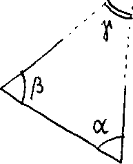
б = 75° Ii3' 32", with S_Q = 3" , are observed .

p

Also, assume that a and 3 are independent, i.e. = 0.

Figure б.T

Let us estimate the third angle у , along with its standard

error S .as follows: Y

у = 180° - (a + В) = 72° 1» "08 _;

s² = <f* )² s² ₊ ф² s²

^{= (-1)2 . (hf 4- (~l)2. (3)2 = 16 + 9 = 25 ,}

that is: S = 5" • Y

Figure 6.3 shows a levelling line between two bench marks

A, С, with observed level differences h. of the individual * i

sections with length i = 1, 2, . . ,^ s. Assume that all the tu's are unc or related and the MSE of h^ is propor- to 2

tional to ft, _a i.e. S, = к £. , where к is a constant. l h.. ■ l

l

Let us deduce the expression for the MSE of the overall level difference ДН between A and С where:

AH = Н_л - H = E h. .

С A ... l 1=1

The mathematical model in this case is

AH = h + h + h₀ + . . . + h -

12 3 s

Hence:

_q2 _ /ЭАН^2 „2< ,ЭДН*2 _q2

AH " ⁽3h₁⁾ \ ^{+ (}Bh₂^} % +

= (l)² (kA₁) + (I)² (k£₂) +

s s

E к £. = к Z £. ,

. l l

1=1 1=1

which means that the MSE of AH equals to the constant of propor­tionality к multiplied by the total (overall) length of the levelling line A — C.

лЛ7-

Let us consider the example 6.3 and assume that the errors in а, Ъ are uncorrelated i.e. S = 0 as we did in Example 6Л. Then we can treat d and at separately (if we are interested in their individual MSE's alone) and we get by applying the law of propagation of errors:

_s2_{= (}M_{)2 s}2₊ ^2 _s2 ₌ 1^2 ₊ ^

d Эа а 9b b a^ a b ⁹

₀2 /Эах2 _c2 ^ ,Эои2 _c2 -2_а2 ^ 2_C2 S = (—) S + (—) S„ = b S + a S- .

а 3a a ЭЪ b a b

Note that the same results can be obtained from Example 6.3 immediately by

putting S _ = 0. ab

On the other hand, if we are interested in the covariance S _

³ da

between the two derived quantities d and ОС , we have to apply the covariance law (equation 6.15) and we will end up with

s ' = Щ- (s ² + a.²) ,

da da b

that is Ф 0, and Z^. (X = (d, a)) is not a diagonal matrix, even though

the of the primary multisample is diagonal i.e. S ^ = 0, see the

results obtained in Example 6.h . This is a very important discovery and

should be taken into consideration when using the derived multisample

X = (d, a) for any further treatment in which case we cannot assume that

d and a are uncorrelated any more and we must take the entire E into

account.

Example 6.7: Let us solve Example 6.2 again, but this time we will consider the primary multisample L = ^i*^2⁵^3^ ^aS uncorrelated and its Z is:

3 0 0 0 3 0 о 0 k

= diag (3, 3, k)

From example 6.2 we have:

В =

10-3 2 10 and X =

Hence:

^zx ^{_ be}l^b ;

3 0 0 0 3 0 0 0 ^

^Ex =

10-3 2 10

-
	1	2
	0	1
J	-3	о e

s s

^Xl ^X1^X2

2

S S

^X2^X1 ^X2

39 6
6 15.

which again verifies the fact that even when 2^ is diagonal

the Л is not •

x.

On the other hand we can treat x^ and x^ separately by using

the law of propagation of errors (since L is uncorrelated) 2 2

to get S and S separately; for instance ,

^Xl ' ^X2

^b2x₁-^^>2b2»1⁺⁽5^{)2 S}\⁺⁽5^{)2 S}\ = (l)² (3) + (о)² (3) + (-3)² (U)

= 3 + 0 + 36 = 39,

ikg

Example 6,8:

which is the same value as we got Ъу applying the covariance law above.

To determine the two sides AC = z and ВС = у of the plane triangle shown in Figure-6.H, the length AB = x along with the two horizontal angles a and 3 were observed and their estimates were found to be:

x = 10 in, with S = 3 cm, x

a = 90° , with S = 2 " , 3 = ^-5° , with S_Q = U" ;

S _n = -1 arc sec and S = S _n = 0 . аЗ ха хЗ

It is required to compute the statistical estimates for

у and z along with their associated variance-covariance

matrix 2^ in cm², where

X = (y, z).

First, we establish the mathematical model which relates the primary and derived samples , i.e.,

X = F (L), where L * (£_1Э£₂,£₃) = (а, 3, x) э

X = (x , x₂) = (y, z) •

From the sine law of the given triangle we get: T _ z. ••■ _ X

sm a sm

sm у

however the angle у is not observed, i.e. it is not an element of the primary sample, therefore we have to sub- stitute for it in terms of the observed quantities, say a and 3 by putting

sin у = sin (a + g),

and we get:

_ sin a

z = x

^{J X} sin (a + 3) ^y

sin 3

sin (a + 3) By substituting for a, 3 and x, we get

у = 10 V2 = 10 (l.UlU) = Ik.Ik m _;

z = 10 m.

Our mathematical model then can be written as:

X = ■

У (a, 3₅ x) z (a, 3, x)

x sin a/ sin (a + 3) x sin 3/ sin (a + 3)

To compute Z = В Z В we have to evaluate the matrix X L

В =

B-which-, is of the form

9£
Эа '	33	' Эх
3z	3.z	_3z
3a '	36	' Эх

sin(_a + g)

tan (a + 3) x

-z

tan (a +3)

JL

sin (a'■+ 3)

_z

x

From the given data, the matrix Z takes the form

s2 a	SaB	S ax
8a		S0x.
S xa	Sx8	<

k	-1	0
-1	16	0
0	0	9

(it is very important to maintain the same sequence of the elements of the primary sample in "both matrices В and E

J_j

to give a meaningful E .)

Now matching the units of the individual elements of В and

2

E з keeping in mind that E is required in cm , results in scaling the В matrix to

z (100)

■y(ioo)

p" sin(a + 3) p^fftan(a + 3)

У

x

В =

-z(lOO)

y(ioo)

pⁿtan(a + 3)

p"sin(a + 3)

X

where p^,f = 20б2б5 = arc sec

В =

Evaluating the elements of the above В matrix we get: 0.007 0.007 l.UlU 0.005 0.010 1.000 and consequently

.007 .005

.007 ,010

1.U1U

1.000

k -1 о -1 1б о

0 0 9

"1

г

.007 .005

.007 .010

l.klk 1.000

1. е.

18.0009 12.7272 12.7272 9-0016

18 13 13 9

cm

and

S = /18 = k.2 cm ;

У

S = /9 = 3 cm. z

The results of the above example show that the high precision in measuring the angles a and 3 has insignificant effect on the estimated standard errors of the derived у and z lengths as compared to the effect of the precision of the measured length x. Hence, one can use the error propagation to detect the main deciding factors in the primary sample on the accuracy of the derived quantities and decide on the needed accuracy of the observations. This process is usually known as pre-analysis which is done before taking any actual measurements by using very approximate values for the observed quantities. This results in accepting specifications concerning the observations techniques to achieve the required accuracy. Some more details about it are given in section 6.3.5­

б. 3.3 Propagation of Non-Random Errors, propagation of Total Errors

The idea of being able to foretell the expected magnitude of

the MSE (as a measure of random errors) of a function of observations -this is essentially what the law of propagation of errors is all about -is often extended to non-random errors. These non-random errors are sometimes called systematic errors, for which the law governing their behaviour is not known. Hence, the values of such non-random errors used in the subsequent development are rather hypothesized (postulated) for the analysis and specification purposes.

The problem may be now stated as follows: let us have an explicit mathematical model

x = f (L)

(6-19)

in which x is a single quantity, f is a single-valued function and

L = (I , %_{0 5} •.• , I ) is the vector of the different observed quantities

that are assumed to be uncorrelated. We are seeking to determine the

influence of small, non-random errors 6£. in each observation I. on the

i l

result x, This influence will be denoted by 6 •

⁴⁷ x

The problem is readily solved using again the truncated Taylor¹ s series expansion, around the approximate values L° = (£°, &°, £°) ,

a. cL s

from which we get:

x

= f(L°) +

9_f

3L

о

L = L

+ Z i=l

ЭЛ.

(6-20)

i i

By substituting 5Z. for (£.-£?) and б for (x-x°) in equation (6-20]

1 11 X

we get:

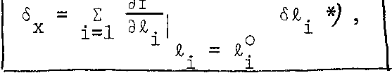
(6-21)

which is the formula for the propagation of non-random error.

Note in formula (6-21)> the signs of both the partial

Э f

derivatives (ттт) and the non-random errors 6£., haveto be considered.

d£l i

(Compare this to formula (6-l8) .)

We may also ask what incertitude can we expect in x if the

observations £. are burdened with both random and non-random errors.

1

In such a case we define the total error as :

т. = /(б² + s²;

(6-22)

with 6 being the non-random error and S being the MSE. Combining

the two errors in x as given above and using equations (6-18) and (6-21)

we get:

1 l-l 1

i-1 Э£. Э£. v у 7 i J

_{= /[ U(|f")2(6£2+S2)} ■+ I ff~ff~ 6£. <$£.]}

1 = 1 ^{1 1} .1=1 ¹ J

or

(6-23)

1

* For the validity of the Taylor's series expainsion, we can see that the requirement of 6£^ being small in comparison to £, is obviously essential.

where q may be regarded as a kind of "covariance" between individual non-random errors, and T. is the total error in the observation £..

As we mentioned in section U.2, the non-random (systematic) errors may he known or assumed functions of some parameters. In this case their influence 6^ on x can he also expressed as a function of the same parameters.

Example 6.9: Let us solve Example 6.2 again considering the primary

multisample L e (&_^₉ % ) to he uncorrelated with variance-

covariance matrix:

о 0 3 о

0 h

and having also non-random (systematic) errors given as: 6L = (6Z_±, 6£₂, Si ) = (-1.5, 2, 0.5), in the same units as the given standard errors.. It is required to compute the total error in the derived quantities: x^ and л according to the mathematical model given in Example 6.2.

The total errors are given Ъу equation (6-22) as:

T = /(<5² + S² ) , ^Xl ^Xl ^Xl

T = /(S² + S² ) ^X2 ^X2 ^X2

We have:

The influences 6 and б - due to the given non-random errors ^Xl ^X2

in L are computed from equation (6-21) as follows:

3 Эх 1 ¹--^L l

= (lX-1.5) + (0)(2) + (-3)(0.5). = -1.5 + 0 - 1.5 = - 3 ,

3 Эх

6 = £ -r~ Si.

*₂ 1=1 3Ji_i l

= (2)(-1.5) + (1)(2) + (0)(0.5) = -3 + 2 + 0 = -l.

Hence, the required total errors will be:

T = 4-ЗГ + 39] = /[U8] = 6^23 , ^xl

T = /[(-l)² + 15] = /[16] = k. ^X2

Example 6.10: Consider again Example 6.6. In addition to the given

information, assume that each height difference lb has got

a non-random (systematic) error expressed as 6 = k'h., ^ h. i

where k^f is another constant ₅ a constant of proportionality

between h. and 6. . Determine the total error in ЛН where i h.

i

s

ЛН = H -Н_л = Z h. = h- + h_n + ... + h .

С A _i=1 l 1 2 s

The total error in ЛН is given by:

^тдн = ^/(бдн ^{+ З}дн^} •

In Example 6.6, we found that: 2

^SAH " ^k ^AC

s

■where к was a constant and I = £ A. is the entire length of

^A^ i=l ¹

the levelling line AC.

We can now compute 6 as follows:

о = £ tt— 6h. _э

ЛН ^₌2. i

i

where

ЭДН ₌ ЭЛН ЭЛН

3h. 3h₀ 3h

12 s

and

6, = k^rh. h. l

i

Then we get

s s

6_A = £ - £ h. = k^! AH.

^ли i=i : * i=l ^х

Finally, the expression for the total error in ЛН will be:

6.3.^- Truncation and Rounding

In any computation we have to represent the numbers we work with , which may be either irrational like it , e, /2, or rational with very many decimal places like 1/3 , 5/ll₅ etc. , by rational numbers with a fixed number of figures.

The representation can be made in basically two different ways. We either truncate the original number after the required number

of figures or we round off the original number to the required length.

The first process can be mathematically described as:

a = a^ = Int (а-10^П)/10^П

(6-24)

where a is the original number assumed normalized*), n is the required number of decimal places and Int stands for the integer value. Example 6.11: тг = 3 • 1^-1592 , n = 3 and we get:

tt = тг = Int (tt-10³) ICf³

= Int (31¹+1.592 ... ) 10~³ = 3lkl • 10"³ = 3.1**!у

The second process ₉ i.e. the rounding-off, can be described

by the formulae:

a =

= Int (a-10ⁿ + 0.5)/Ю^П

(6-25)

in which all terms are as described above. Example 6.12: tt, n = 3 and we get:

R

= Int (тг-10³ + 0.5) Ю"³

^-3

тг = 7t

= Int (3141.592 ... + 0.5) 10 = Int (3142.092 ...) 10~³ = 3142 • 10"³ = 3.142.

* To normalize the number, say 3456.21, we write it in the form 3.45621

It can be seen that the errors involved in the above two alternative processes differ. Denoting the error in "a" due to

truncation Ъу б and the error due to rounding 'by 5 , we get;

б = a

- e [0, 10"ⁿ)

б = a - a,, e [-0.5 10~ⁿ, 0.5 10^_n)

and we may postulate that б has a parent random variable distributed according to the rectangular (uniform) PDF (see section 3.2.5):

R(0.5 10~^П, 0; 6 ) (6-26)

while б has parent PDF:

R(0, а; б ) (6-27)

as shown in Figure 6.5.

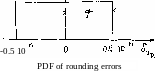
Figure 6.5

1бО

From example 3.17 ₉ section 3.2.5 we know that a = q//3, where q equals half of the width of the R. In our case, obviously q = 0.5 10~^П so that a = 0.289 10"ⁿ.

Because of their different means, the error in truncation propagates according to the "total error law" and the errors in rounding propagates according to the "random error law". Hence, if we have a number x:

x = f,(L) , (6-28)

where

L = () , i = 1, 2, ... ,s

is a set of s numbers to be either truncated or rounded off individually, we can write the formulae for the errors in x due to truncation and rounding errors in the individual £^s as follows:

s 2

6_x = /[ E (|f-) -± Kf²ⁿ] . (6-30)

^ХБ i-1 ^3£i ^ ¹²

This indicates clearly that the error in x due to the rounding process

is less than the corresponding error due to truncation; and this is

why we always prefer to work with rounding rather than truncation.

Example 6.13: Let us determine the expected error in the sum x of

1000

a thousand numbers a«.x = . E_ a,, if

V i=l 1

(i) the individual values a^ were truncated to five decimal places;

(ii) the individual values were rounded-off to five

decimal places.

Solution:

(i) The error б due to the truncation of individual a ^XT

computed from equation (6-29) as follows: 1000 ■

^XT i=l ^dai

¹⁰⁰⁰ _a ²

^{=/{[0.5 • io"5 • io3]2+ ^1 • io"10- 103}}

О

= /{10 (2500 + 0.833)}

= 0.005001 = 0.005 •

(ii) The error б due to the rounding of individual a.

computed from equation (6-30) as follows:

1000 . 2 . _in

x_{R i=1} 3a. 12

= /{(1000) (y| • 10^-10)}

= /{10^-8 (0.833)} = 0.000091 , which is much smaller than the corresponding б

^XT

1б2

6.3.5 Tolerance Limits, Specifications and Preanalysis

Another importantant application of the propagation laws for errors is the determination of specifications for a certain experiment when the maximum tolerable errors of the results, which are usually called tolerance limits , are known beforehand. Such process is known as pre-analysis. The set-up of the specifications should therefore result in the proper design of the experiment, i.e. the choice of observation techniques, instrumentation, etc. , to meet the permissible tolerance limits.

The specifications for the elementary processes should account for both the random and the inevitable non-random (systematic) errors. This is, unfortunately, seldom the case in practice. It is usual to require that the specifications are prescribed in such a way as to meet the tolerance limits with the probability of approximately 0.99- If we hence expect the random errors to have the parent Gaussian PDF, the actual results should not have the total error, composed of the non-random error 6 and 2.5 to 3 times the RMS , which corresponds to probability of 99% ,larger than the prescribed tolerance limits, i.e.

(6-31)

T < A& + (3a ) } .

Example 6.1k: Assume that we want to measure a distance D = 1000 m,

with a relative error (see U,10) not worse than 10 \ using a 20 m tape which had been compared to the "standard" with a precision not better than 3c < 1 ram , i.e. tolerance limits of the comparison were + 1 ш , Assume also that the whole length D is divided into 50 segments d^, i = 1, 2, . . . , 50,

each of which is approximately 20 m. Providing that each segment d^ will he measured only twice: forward F_^ and backward , what differences can we tolerate (accept or permit) between the back and forth measurements of each segment? Solution:

The tolerance limits in D, i.e. the permissible total error in D, is given by

T_D = 1000щ 10 = 0.10 ш = 10 cm.

This total error T^ is given by

^TD = ^/{6D ^{+ ( 3}°D^)2} > where 6^ is the non-random (systematic) error in D, is the random error in D and the factor 3 is used to get probability > 99% according to the assumed Gaussian PDF. Knowing that 50

D = Z d. , where d. = 77 (F.+B. ) ,

i—1 i i i i

we get:

50 _3D ⁶D ⁼ А Ж ^6di >

1=1 i

where

3d. 3d.

1 1

_{= 77 5F. + j SB. = j (6.+6. ) = 6. .}

2 l 2 l 2-1 l l

Hence.

50

6^ = £ 1*6.< 50 mm = 5 cm.

cm

Thus, we must require that:

2

^(3oD^} -^TD " ⁶D ^{= (10)} -^{(5) = 75}

or

2 ^ 75 cm² 2

Op <^ —^ ²² 0.33 cm

in order to meet the specifications.

Denoting the MSE in the individual segments d^ Ъу

°d ~ °d ^^a^^" ^assume(i equal) ve get

₂ 5° ₂ 2

°» " _±l_x V = ⁵°°d •

from which we obtain 2

2 ^ °D 8.33 _л 2

Remembering that each segment d^ is given by:

^di-2 ^(Р1^+В1> •

and denoting the MSE in either or (both assumed equal) Ъу о ve get:

2 2 / i \ 2 , / i \ 2

3d. ² _л.' 3d. 2

a

d. d ^X3F.' P. ЭВ. B.

1 1 1 1 x

,1x2 2 _,_ ,1ч² 2

= (g) о + (-) a

and

/1 . 1\ _2 1 2

= ⁽¥ ⁺ ^ ^CT - 2 ⁰

а² < 2а² = 2(0.lZ) = 0.33 cm. —. £

Recalling that we want to know what differences between the forth and back measurements can we tolerate, and denoting such differences by Д^, we can write:

Д. = F.-B. .

i ii

Then:

2 2 / i \ 2 , / i \ 2

V = ^ад ^{= (}эЁГ⁾ V ⁺⁽эвГ^{) а}в. i iiii

(ifa² + (-1)²а²

= 2а²

Thus, we end up with the condition:

a² <_ 2a² = 2(0.33) = 0.66 cm²

or

а_д _< 0.816 = 0^ cm.

This means that if we postulate a parent Gaussian PDF for the differences A, the above Од is required to be smaller or equal than the RMS of the underlying PDF. Consequently, the specifications will be as follows: We should get of the differences Д¹ s with _+ а_д, i.e. within +_ 0.8 cm, and 95% of Д within j+ 2Сд, i.e. within + 1.6 cm. These specifications are looser than a man with an experience in practice would expect. It illustrates the fact that in practice the specifications are very often unnecessarily too stringent.

6Л Problem of Adjustment 6.H.1 Formulation of the Problem

Let us resume now at the end of section 6.2 where we have defined the proper problem of adjustment as the transition

(L, E_L) + (X, E_x) (6.32)

for an оverdetermined mathematical model

F(L, X) = 0 . (6.33)

By "overdetermined" we mean that the known L contains too many components to generally fit the abbve model for whatever X we choose, i.e. yielding infinite number of solutions X . The only way to satisfy the model ? i.e. the prescribed relations_;is to allow some of or all the L to change slightly while solving for X. In other words, we have to regard L as an approximate value of some other value L which yields a unique solution X and seek the final value L together with X.

Denoting

L - L = V (6.3*0

we may reformulate our mathematical model (6.33) as:

F(L, X) = F(L + V, X) = 0 (6.35)

where V is called the vector of discrepancies.

Note that V plays here very much the same role as the v's have played in section h.8. From the mathematical point of view, there is not much difference between V and v. However, from the philosophical viewpoint, there is, because V represents a vector of discrepancies of

s different physical quantities (see also section 5•h)while v was a vector of discrepancies of n observations of the same physical quantity. To show the mathematical equivalence of these two we shall, in the next section, treat the computation of a sample mean as an instructive adjust- ment problem. - '

6Л.2 Mean-of a/Sample as an Instructive Adjustment problem^weights

Let us regard a random sample L = (&^, . . .₅ of n

observations representing one physical quantity Л as uncorrelated estimate of the mean . Further we shall denote the definition set of L by L, where L = (1 ₉ I , . . •> &_m) consists of only m. distinctly different

A

values of £^Ts. Let us seek an estimate x, satisfying the mathematical model

x = l (б.Зб)

representing the identity transformation. Evidently, the model is over determined because the individual 1L , j = 1, 2, . . .^m, are different from each other and cannot therefore all satisfy the model. So, we reformulate the model as:

x = 1. + v. j = 1, 2, . . ., m (6.37)

J J

where the v^fs are the discrepancies. We have to point out that, although we seek now the same result as we have sought in section k.J, the formu­lation here will be slightly different to enable us to use analogies later on. While we have been taking all the n observations into account in section H.7, we shall now work only with the m distinctly different values 1.,

j = 1, 2, . . .>т, that constitute the sample L*J.

Thus we shall have to compute the mean I from the second formula introduced in section 3.1.3 (equation (З^Ж i-e.:

i = p(ip⁼ J_x *j ^pj > ⁽⁶*³⁸⁾

rather than the first (equation (3.3)) as used in section *t.T. Here, according to section 3.1.3, Pj = c^/n with c^, being the count of the same values £*' in the original sample L* containing all n observations •

и

Hence P. are the experimental (actual) probabilities• In other words, if

j

we wish x to equal I, the model (6.37) yields the following solution:

m

x - Z I. P, _; (6.39)

J=l ^{J 3}

or

^л Ф — x = P L

(6Л0)

in vector notation, where P « (P^, Pg, .P^)•

* L =(£,£, * . £ ) can be regarded in this context as a sample of "grouped" observations, i.e. each constituent £ » j = 1, 2, . . ,,m, has a count ( frequency) с . associated with it in the original sample

L . ^J

The coefficients P^ are called weight coefficient^ or simply weights ^and x is called the weighted mean - analogy borrowed from mechanics (see section 3.1.3). Note that , with the weights being nothing else but the experimental probabilities, we put "more weight^fr on the values with which we are more "certain", i.e. which are repeated more often in the sample, which is intuitively pleasing.

In our slightly different notation even the least-squares prin­ciple, as formulated in section 5*3, would sustain a minor change. While we were seeking such £° as to make

1 ^П 2 1 ^П о 2

i E v = i ,£ (£ - £ ) (6.41)

n i n 1=1 i

1=1

minimum, we would have to write now the condition of minimum variance as:

m

min [ £ P.v. ] , (6.42)

_яо j==l ^{3 3} ~

£ £ R ^J

where v. = £. - £°. In matrix notation, (6.42) becomes:

T

mm V PV

о

£ eR

(6.43)

where P is a diagonal matrix, i.e.

P = diag (P , P₉, , P ) . (6.44)

JL ~> m

The latter formulation, i.e. equations 6.42 and 6.43 is more general since we can regard the former formulation, i.e. euqation 6.41 as a special case of (6.42) and not vice-versa. We have

i ; 2 ; ^ 2

— E v. = I P.v. n . . i . _ 11

1=1 1=1

which implies that P^ = for i = 1, 2, .. ., n are equal weights for all the observations £^. Hence we shall use (6.43) exclusively from now on. The same holds true even for the two formulae for £ and we shall use equation (6.40).

Note that once we apply the condition 6.43, the discrepancies cease to be variable quantities and become residuals (see 4.8). We shall denote these residuals by V.

Equation 3.7 can nov Ъе obviously written as

(6Л5)

or in matrix notation,

2 ^ЛТ ^л S_T = V PV .

(6Л6)

Consequently, we shall restate the least-squares principle as follows:

T

the value x that makes the value of the quadratic form V PV the least ensures automatically the minimum variance of the sample L. This property does not depend on any specific underlying PDF. If L has got normal parent PDF (or any symmetric distribution), x is the most probable estimate of x, which is sometimes called the maximum likelihood estimate of x.

6Л. 3 Variance of the Sample M-ean

We have shown that the simple problem of finding the mean of

a sample can be regarded as a trivial adjustment problem. Hence we are entitled to ask the question: What will be the variance-covariance matrix of the result as derived f**om the variance-covariance matrix of the original sample ? In other words, we may ask what value of variance can be assoc­iated with the result - the mean of the sample.

The question is easily answered using the covariance law (section 6.3.1). We have established that (equation 6Л0) :

T"~

x =P L .

Hence, by applying the covariance law (equation 6.15)we obtain:

Е = BE -В = Р Е -Р = S* х L L х

i.e.

= P^TZ-P . (6.47) x L

Here E- is not yet defined. All we know is that L = (£- , ]L,. . Jl )

L 12m

is a sample of "grouped" observations with different weights (observed probabilities) P^ associated with them. Let us hence assume these obser­vations uncorrelated and let us also assume that there can be some 2

"variances" S- attributed to these observations. In such a case, the variance covariance matrix of L can be expressed as

E£ = diag (s| , s| , s| ) . (6.48)

1 2 m

Substituting (6.48) into (6.47), we get:

2 ^Ш 2 2

S- = E P. S - *) . (6.49)

x . j £.

3=1 1

On the other hand the value of x (i.e. the sample mean) can be computed using the original sample of observations, L = (£^, l^, ..., £^) , i.e. the ungrouped observations £^, i = 1, 2, ..., n, which all have equal experimental probabilities (equal weights) of 1/n, yielding: n

x = - E £. = - [A, + A- + ... + A ] . (6.50)

n . , i n 1 2 n

i=l

2

Hence, we can compute the variance of the mean, i.e. S^, again by applying the law of propagation of errors on (6.50) , and we get:

о ⁿ av 2 о ₁ 2 n

_{3Л = A <fl7> S £ " Ф A S£. ' (6'51)}

*It should be noted here that since L = (£^, 1L/ • • • ' A^) is a sample of group observations, for which a different weight Pj (experimental proba­bility) is associated with each element £., j = 1, 2, ..., m, the individual variances S - assigned to the £. are, in""* general, different from each other, i.e. they j vary with the groups of observations.

x 1=1 l ! i=l i

in which all the 'variances! are again assumed to have the same value

¹ 2

and equal to the sample variance S given by

- ±- S U. - x)². (6.52)

1 = 1

S? = -₂ (n S²) = S²/n x n

Equation (6.51) then gives:

(6.53)

which indicates that the variance of the sample mean equals to the variance

of the sample computed from equation (6-52) divided by the total number

of elements of the sampled

We thus ended up with two different formulae, (6.U9) and

(6.53)₅ for the same value S^. In the first approach, we have regarded

x

the individual observations (really groups of observations having the same

2

value) as having different variances S - associated with them. The second

j

approach assumes that all the observations belong to the same sample with

2 2

variance S . Numerically, we should get the same value of S_A from both

^L x

formulae, hence

m _s2

E (P.² S²» ) = -± . (6.5h)

j=l ^J, h ⁿ

Let us write the left hand side, of (6.5*0 in the form:

m m

* In terms of our previous notation, we can write the variance of the sample mean as

S = Sfy n .

£ ^L

1 (P S- ) = E [P.(P Sf _)} ■J=l ⁵ *j j=l ^{3 3} V^J'

and the right hand side in the form:

2 2

S_ n S_

ll 1^ X7 1 / Jj 4

n ~" n ~* n 1=1

Using the same manipulation as in section 6Л.2 when dealing with the V^T s and Х'з, and also earlier, in section 3.1.^ when prooving equation

(3-Mj the right hand side can he rewritten as:

2 2

n S m S

i S (-±4 =. Z [P. (—)] , n n in

i=l j=l ^J

in which P. has the same meaning as in (6.U9).

J

Now, the condition (6.5*0 becomes:

a²

m m S

Z [P.(P. S²: )] = E [P. (-f)], (6.55)

j=l ^{J J} j 3=1 ^{J П}

which can be always satisfied if

" S²

Pj s| = -j± = K, j = 1, 2, . . . , m, (6.56)

J

where К is a constant value for a specific sample that equals to the variance of the sample mean. From (6.56) we get:

⁸^ ⁼ Pj ⁵ , j =1, 2, ... ,i, (6.57)

which shows that in order to get the correct result from {6Л9) we have to assume that in the first approach the individual observations have

variances inversely proportional to their weights.

This result is usually expressed in the form of the following principle: the weight of an observation is inversely proportional to its variance, i.e.

We can also write using equation (6.57):

P = P₂S^ = ... = rS²_Q = К (6.59)

2

where S_Q, constant for a specific sample, is known as the variance of unit weight. It can be interpreted as the variance of an imaginary observation whose weight equals to one. In the case of sample mean I, S_q equals to S-. From equations (6.46) and (6.53) we can write: 2 V PV

S* = . (6.60)

x n

This result will be often referred to in the subsequent development.

We have to point out that the whole argument in this section

2 2

hinges on the acceptance of the "variances" S and S - . They have been

1 1

introduced solely for the purpose of deriving formulae (6.53),(6.58) that are consistent with the rest of the adjustment calculus. . The more rigorous alternative is to accept the two formulae by definition.