In the interval [6,10] is nine. This number

represents (т~).100% = 36% of the sample.

Or, we say that the actual probability

P(6<x<10) = 0.36, which does not agree precisely

with the result obtained when using the

corresponding histogram (i.e. 0.27).

The difference between the actual probability and the computed probability using the histogram, as experienced in example 3.12, is largely dependent on the chosen classification of the<sample (selection of the class-intervals). Usually, one gets a smaller difference (better agreement) by selecting the class-boundaries so as not to coincide with any of the elements of the given sample. The construction of histograms can be considered a subject of its own right. We are not going to venture into this subject any deeper.

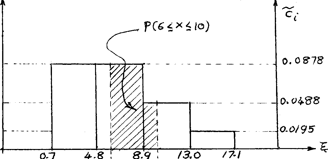
Example 3.13: If we, for instance, use the following classification (for the sample £ given in example 3.10): [0.7, 4.8], [4.8, 8.9], [8.9, 13] and [13, 17.1], i.e. we have again four equal intervals, for which A = 4.1. Then we get the class-counts as c^ = 9, c^ = 9, c^ = 5 and = 2. The quantity пЛ = 25.4.1 = 102.5. Hence, the relative counts are:

VVII?I 0-0878'

⁵з - ik? * °-⁰⁴⁸⁸' vib'⁰-⁰¹⁹⁵-

In this case, the new histogram of the sample £ is shown in Figure 3.5.

i i

6 to

Figure 3.5

The probability P(6<x<10) is computed as follows (shaded area in Figure 3.5)* P(6<x<10) = P(6<x<8.9) + P(8.9<x<10)

= 2.9.0.0878 + 1.1.0.0Ш =

= 0.25U6 + 0.0537 =

= 0.3083 = 0.31, which gives a better agreement with the actual probability than the classification used in example 3.11.

Relative frequency

Ul

The graphical representation of a histogram, which uses the central point of each box (class-midpoint) and its ordinate (the corresponding relative class-count), is called a polygon.

In order to make the total area under the polygon equal to one we have to add one more class interval on each side (tail) of the corresponding histogram. The midpoints s¹ and &^! of these two, lower and upper tail intervals,are used to close the polygon.

Therefore, it can be easily seen that the area a* under the poly­gon has again the properties of probability. This means that a' is one of the possible PDF^Ts of the sample. Hence a^! can be used for determining the probability of any-D^f * [a,, b]c[s.\1¹J . Note also here that the ordinates of the polygon do not represent probabilities.

Example 3>lU: The polygon corresponding to the histogram of Figure 3.U is illustrated in Figure 3.6,

h2

Similar to the histogram, the area"aⁿunder the polygon should be equal to one. To show that this is the case, we compute^f!a^tTusing Figure 3.6 as:

a = 1+ (| . 0.12 + |- (0.12 + 0.08) +

+ ~ (0.08 + 0.03) + | (0.03 + 0,02) + + - . 0.02) = 2(0.12 + 0.20 + 0.11 + 0.05 + 0.02) = 2 (0.50) = 1.00. Let us compute the probability P(6<x<10) using the polygon (the required probability is represented by the shaded area in Figure 3.6). To achieve this, we first have to interpolate the ordinates corresponding to 6 ' and 10, which are found to be 0.090 and 0.0^25, respectively. Therefore, the required probability is: P(6<x<10) = P(6<x<7) + P(7fx<10)

= 1.1(0.09+0.08)+3.~(0.08+0.0^25) = 1.0.085 + 3.0.06125 = 0.085 + O.lQk = 0.27, which is the same as the value

obtained when using the corresponding histogram.

So far, we have constructed the histogram and the polygon corresponding to the PDF of a sample. Completely analogously, we may construct the histogram and the polygon corresponding to the CDF of the sample which will be respectively called the cumulative histogram and the cumulative polygon. In this case, we will use a modified form of equation (3.2), namely

C(a) = P(x<a) = I P(x <x<x ) • (3.lU)

x. <a

Example 3.15: Let us plot the cumulative histogram and cumulative polygon of the sample £ used in the examples of this section.

For the cumulative histogram, we get the following by using Figure 3.U:

C(l) = P(l) = 0 (remember that the probability of individual elements from the histogram or polygon is always zero).

C(5) = P[l,5] = U.O.12 = 0.U8, 0(9) = C(5)+P(5,9l = 0.U8 + U.O.08

= 0.U8 + 0.32 = 0.80, 0(13) = C(9)+P(9,13] = 0.80 + U.O.03

= 0.80 + 0.12 = 0.92, C(.1T) = C(13)+P(13,17] = 0.92 + U.0,02

= 0.92 + 0.08 = 1.00. Figure 3.7 is a plot of the above computed cumulative histogram.

kk

CCfil

For the cumulative polygon, we get the following by using Figure 3.6: C(-l) = 0,

C(3) = P[-l,3] = |(U.o;i2)= |(0.U8)= 0.2U, C(7) = C(3)+P(3,7J = 0.2k+ |.U(.0.12 + 0.08)

= 0.2U + 0Л0 = 0.6k, C(ll) = C(7)+P(7,ll] = 0.6k + |Л(0.08 + 0.03)

= 0.61+ + 0.22 = 0.86, G(15) = C(ll)+P(ll,15l = 0.86+ I .40.03 + 0.02)

= 0.86 + 0.10 = 0.96, C(19) = C(15)+P(15,19] = 0.96 + I . U.O.02

= 0.96 + 0.0k = 1.00 Figure 3.8 is a plot of the above computed cumulative polygon (note here, as well as- in Figure 3.7» the properties of the CDF mentioned in example 3.k).

1*5

_{CO?) I}

By examining Figures 3.7 and 3.8, we can see that the cumulative

polygon uses the central point of each class-interval along with its ordinate from the corresponding cumulative histogram. Therefore, the relationship between the cumulative polygon and its corresponding cumulative histogram is exactly the same as the relationship between the polygon and its corresponding histogram.

Because of the nature of the CDF, we can see that the cumulative probability - represented by an area under the PDF extending to the left­most point - is represented just by an ordinate of the cumulative histogram or the cumulative polygon. Hence the cumulative histogram or the cumulative polygon can be used to determine the probability P[a,b], a<b, simply by subtracting the ordinate corresponding to a from the one corresponding to b.

Example 3.1б; Let us compute the probability P[6,10] by using:

(i) the cumulative histogram of Figure 3.7,

(ii) the cumulative polygon of Figure 3.8, First, we get the following by using Figure 3.7* The interpolated ordinates corresponding to 6 and 10 are found to be O.56 and 0.83, respect- ively. Therefore, P[6,10]= P(6<x<10) =

= О.8З-О.56 = 0.27, which is the same value as the one obtained when using tlie histogram (example 3.12).

Second, we get the following by using Figure 3.8: The interpolated ordinates corresponding to 6 and 10 are found to be 0.5^ and 0.805, respectively. Therefore: P[6,10]= P(6<x<10)= 0,805-0.5^0.27 , which is again'^: Шё same value as the one obtained when using the polygon (example 3.lU). To close this section, we should point out that both the histo­grams and the polygons (non-cumulative as well as cumulative) can be refined by refinning the classification of the sample. Note that this refinement makes the diagrams look smoother.

47а

3.2 Statistics of a Random Variable 3.2.1 Random (Stochastic) Function and Random (Stochastic) Variable

In order to be able to solve the problems connected with inter­val probabilities (see the histograms and polygons of section 3.1.6) more easily and readily, the science of statistics has developed a more con­venient approach. This approach is based on the replacement of the troublesome numerical functions defined on the discrete definition set of a random sample, by more suitable functions. To do so, we first define two idealizations of the real world: the random (stochastic) function and the random (stochastic) variable.

A random or stochastic function is defined as a function X mapping an unknown set U* into R, that is

xe {U R}

(Later on, concepts of multi-valued Xe {u -> R^m} (where R^m is the Cartesian m-power of R, see section 1.3) are developed.)

This statement is to be understood as follows: For any value of the argument ueU, the stochastic function x assumes a value x(u)£ R. But, because the set U is considered unknown, there is no way any formula for x can be written and we have to resort to the following "abstract experiment" to show that the concept of random functions can be used.

"Note that in experimental sciences the set U may be fully or at least partly known. The science of statistics however, assumes that it is either not known, or works with the unknown part of it only.

Suppose that the function \x Is realised by a device or a process (see the sketch.) that produces a functional

value x(u) every time we trigger it. Knowing nothing about the inner workings of the process all we can do is to record the outcomes x(u). When a large enough number of values x(u) have been recorded, we can plot a histogram showing the relative count of the x(u) values within any interval [x_q, x^] • In this abstraction we can imagine that we have collected enough values to be able to compute the relative counts for any arbitrarily small interval dx and thus obtain a'smooth histogram¹. Denoting the limit of the relative count divided Ъу the width dx of the interval [x, x + dx], for dx going to zero, Ъу ф(х) we end up with a function ф that maps x e r into r.

Going now back to the realm of mathematics, we see that the outcome of the stochastic function can be viewed as a pair (x(u), ф(х)). This pair is known as the random (stochastic) variable. It is usual in literature to refer just to the values x(u) as random variable with the tacit under standing that the function ф is also known.

We note that the function ф is thus defined over the whole set of real numbers R and has either positive or zero values, i.e. ф is non-negative on all R. Further, we shall restrict ourselves to only such ф that are integrable on R in the Riemannian sense, i.e. are at least piece-wise continuous on R. 3.2.2 PDF and CDF of a Random Variable

The function ф described in 3.2.1, belonging to the random variable x, is called the probability distribution function (PDF) of the random variable. It can be regarded as equivalent to the experimental

PDF (see 3.1.2) of a random sample. From our abstract experiment it can be seen that

ф(х) dx = 1

(3.15)

since the area under the "smooth histogram" must again equal to 1 (see 3.1.6). This is the third property of a PDF, the integrability and non-negativeness being the first two. We note that eq. 3.15 is also the necessary condition for ф(x) dx to be called probability (see 2.1).

Figure 3.9 shows an example of one such PDF, i.e. ф in which the integral (3.15) is illustrated by the shaded area under the ф.

The definite integral of the PDF, ф, over an interval D*c D is

called the probability of D'. So, we have in particular:

/^Х°ф (x) dx=P(x<x_o) _e[0, 1] ,

(3.16a)

oo

/ ф(х) dx = P(x^x_o) £[0, 1] ,

(.3.16b)

X

о

2

/ ф(х) dx = P(x_x 1 x £ x₂) e [0, 1] .

^xl

(3.16c)

Consequently,

P(x > x ) = 1 - P (x < x_Q) .

— о — ^w

(3.17)

The integrals (3.l6a), (3.l6b) and (3.l6c) are represented by the corresponding shaded areas in Figure 3.10: а, Ъ, and с, respectively.

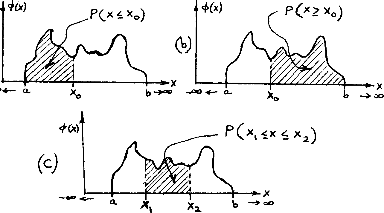
Figure 3.10

At this point, the difference between discrete and compact probabil-

* The whole development for the discrete and the compact spaces could be made identical using either Dirac¹s functions or a more general definition of the integral.

ity spaces, should be again born ^: in.-mind. In the discrete space, the value of the PDF at any point, which is an element of the discrete definition set of the sample, can be interpreted as a probability (section 3.1.2). However in the compact space, it is only the area under the PDF, that has got the properties of probability.* We have already met this problem when dealing with histograms.

Note further that:

P (x = x_q) = / ф(х) dx = 0*) x

о

Analogous to section 3.1.2, the function У defined as

(3.18)

? (x) » / -ф(у) dy, e[x [0, 1]} ,

where yeR is a dummy variable in the integration, is called a CDF provided that ф is a PDF. У is again a non-negative, never decreasing function, and determines the probability P(x £ x ). (Compare this with section 3.1.2); namely:

T(x_Q) =P(x£x_o) e [0, 1] . (3.19)

Figure 3.11 shows how the CDF (corresponding to the PDF in Figure 3.9) would look.

ЧЧ*И

* This may not be the case for a more general definition of the integral, or for ф being the Dirac¹s function.

If ф is symmetrical, ¥ will be "inversely symmetrical"around the axis ^lF(x) = 1/2. Figure 3.12 is an example of such a case.

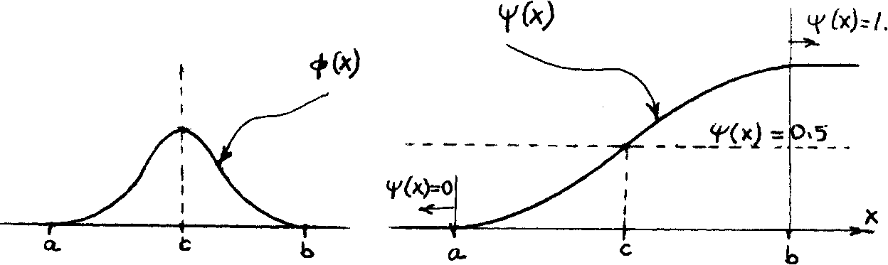
Figure 3.12

Ifefre^th&t ¥ is the primitive function of ф since we can write:

ф(х) = ¹— .

dx

In addition, we can see that ф(х) has to disappear in the infinities in order to satisfy the basic condition :

00

/ ф (x) dx = 1.

Hence, we have:

lim y(x) = 0 * ^lim ^(x) = 1 . ■

3.2.3 Mean and Variance of a Random Variable

It is conceivable that the concept of a random variable is useless if we do not know (or assume) its PDF. On the other hand, we do not have the one-to-one relation between the random variable and its PDF as we had. with

the random samples (section 3.1.1 and 3.1.2). The random variable acts only as an argument for the PDF.

The random variable can be thus regarded as an argument of the function called PDF, that runs from minus infinity to plus infinity. Therefore, strictly speaking, we cannot talk about the "mean" and the "variance" of a random variable, in the same sense as we have talked about the "mean" and the "variance" of a random sample. On the other hand, we can talk about the value of the argument of the centre of gravity of the area under the PDF. Similarly, we can define the variance related to the PDF. It has to be stated, however, that it is a common practice to talk about the mean and the variance of the random variable; and this is what we shall do here as well.

The mean у of the random variable x is defined as:

у = 7 x ф(х) dx ,

:з.2о)

Note the analogy of (3.20) with equation (3.U), section 3.1.3.

у is often written again in terms of an operator E*; usually

we write

CO к

E* (x) = у = / x ф (x) dx .⁺J (3.21)

E* is again an abbreviation for the mathematical Expectation, similar to the operator E mentioned in section 3.1.3. However, we use the "asterisk" here to distinguish between both summation procedures, namely: E implies the summation using £; and E* implies the summation using /.

We can see that the argument In the operator E* is x« ф(х) rather than x, x being just a dummy variable in the integration. However, we shall again use the customary notation to conform with the existing literature.

We have again, the following properties of E*, where к is a constant: (i) E* (kx) = к E* (x);

(ii) E* .E (x^J)=.E E* (x^J), where x^J, j = 1, 2, •.. r,

J"""l J -L

are r different "random variables", i.e. , r random variables with appropriate PDF¹s; (iii) and we also define:

E*(E*(x)) = E* (x) = y⁺⁺). The variance a² of a random variable x with mean у, is defined as:

a² = / (x-y) ф (x) dx .

(3.22)

Note the analogy of (3.22) with equation (3.8), section 3.1.U. The square root of a², i.e. о, is again called the standard deviation of the random variable.

Carrying out the operation prescribed in (3.22) we get:

00

2 2 о

a = f [x ф(х) 2хуф (x) + уф (x)] dx

— CO

CO 00 00

2 2

= / x ф(х) dx - 2y / x ф(х) dx + у / ф(х) dx .

tt

In order to prove this equation, one has to again use the Dirac ¹ s function as the PDF of E*(x).

In the above equation, we know that the integral in the second term equals у (equation (3.20)), and the integral in the last term equals one (equation (3.15)). Therefore, by substituting we get:

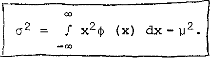
(3.23)

Note the similarity of the first term in equation (3.23) with

m

E(£ ) = £ d. p(d.) (section 3.1.4). This gives rise to an often used j=l J D

notation:

a² = E* (x-y)² = E* (x-E*(x))² . (3.23a)

We shall again accept this notation as used in the literature, bearing in mind that E* is not operating on the argument, but on the product of the argument with its pdf.

The expression

= / x | (x) dx

(3.24)