

2. Fundamentals of the mathematical theory of probability
2.1 Probability Space, Probability Function and Probability
Let us have a set d = 0 and let us assume that it can be partitioned into mutually disjoint subsets d^C d such that d s ud_. (by mutually disjoint subsets we mean such subsets that dJ*) d.. = 0 for any pair d^, d_., i 7* j) . Such a set d we shall call probability space.
Any mapping P of d onto [0, 1] (that is the set of all positive real numbers "b" satisfying the inequalities (0 £ b £ 1)) that has the following two properties:
(1) If d'cd, then P(_d") = 1 - P(d - d1) , (note that d-d1) is the complement of d1 in d; see section 1.5), and
n
(2) If d- , d9, . .., d cd are mutually disjoint, then P( [) d.) =
1 z, n , _ 1
1=1
n
£ P(d.), is called a probability function. The value (P(d*))
i=l x
of the probability function P (takes any value from [0, 1]) is called the probability. Note that the difference between the function and the functional value has been mentioned in section 1.6.
The above two properties of the probability function have the following consequences:
P(P) =1,
P(0) = G,
If d'cd; then p (d1) £ lf
If d"cd\- then P(d") _< P (d1) , and
If A, bcd, and A(\B s 0; then P(a(Jb) = P (A) + P(B) .
If D is a point set , i.e. its elements can be represented by-points , it is always decomposable.
The value Z P(D.) e [0, l] is sometimes called the total or
i
accumulative probability of U D..
i
2.2.a Conditional Probability
If а, Б CD; then the ratio Р(аПВ)/Р(В) = p(a/b) is called the conditional probability. The right hand side, that is P(A/B); is read as "probability of A given B". In other words, the conditional probability P(A/B) can be interpreted as the probability of occurrence of A under the condition that В occurred.
From the above definition of the conditional probability, we notice that:
If P(B) = 0; then P(A/B) is not defined,
If В С A; then А П В = В (see section l.k), and then P(A/B) = 1,
If А П В 5 0 , i.e. A and В are disjoint sets ; then P(A/B) = 0.
.2.3* . Combined Probability ■
If the conditional probability P(A/B) equals to P(A), then it is clear that the occurrence of A does not depend on the occurrence of B. In such a case we say that A and В are independent. Using the definition of the conditional probability from the previous section, we can write:
P(AflB) = p(a) • p(b) , This can be understood as the probability of simultaneous occurrence of A and B, which is usually denoted by P(A, B) and read as probability of A
and В, and known as the combined (compound) probability of A and В, that is
P(A, B) = P(A) • P(B) . Similarlyr we define the combined probability of occurrence of the independent D^, D2> . D^C D as the product of their individual probabilities, i.e.
P(D±, Dj) = P(D±) P(Dj) i 7* j
P(D±, Djf Dk) = P(D±) P(Dj) P(Dfc) j, 35^k, i ^ k,
n
P(D,r Dor D ) = П P(D.) .
12 П . _ i
1=1
Example 2.1: Suppose we have decomposed the probability space D into seven mutually disjoint subsets D^, , .. ., as shown in Figure 2.1 such that:
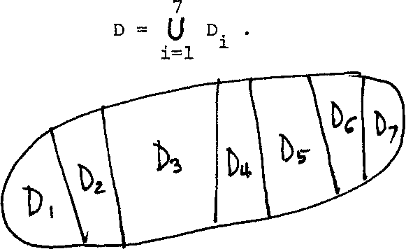
Figure 2.1.
Assuming that the probabilities P(D^) of the individual subsets are found to be:
P(DX) = 1/28, P(D2) = 2/28, P(D3) = 3/28f P(D4)'= 4/28, P(D5) = 5/28, P(D6) = 6/28, and P(D?) = 7/28; then we get:
Total probability of D., i = 1, 2, ..., 7 is
7
P(D) = P(U D.) = I P(D±) = (1+2+3+4+5+6+7)/28 = 28/28 = 1.0.
i 1 i=l
7
Combined probability of all D. = П P(D.) = 0
i , - l 1=1
Example 2.2; In this example we assume that our probability space D is
decomposed into five elements d, e D, j = 1, 2, . .., 5. If the probabilities P(Dj), as represented by the ordinates in Figure 2.2, are given as:
4
PC*)
0/У 0.2-
ол-
I_I
Figure 2.2
P(d ) = 0.2, P(d2) =0.3, p(d3) = 0.1, P(d4) = 0.1,
and P(d_) = 0.3; then we get: b
5
Total probability p(d) = p({Jd.) = l P(d.) = 0.2+0.3+0.1+0.1+0.3
1 3
= 1.0
Combined probability of d^ and d^ (for example) = P(d^f d^)
2
= IT P(d.) = 0.2.0.3 = 0.06.
This combined probability has to be understood as the probability of simultaneous occurrence of d^ and d^ under the assumption
of their independence.
2.4. Exercise 2. We have determined that every number of a die have the probability of appearing when the die is tossed, proportional to the number itself.
Let us denote: A = {even numbers\ , В = ^prime numbers^ , and С = [odd numbersj; all subsets of the set of numbers appearing on the die.
Required: (l) Construct the probability space d.
(2) Find the probability of each individual element d^ e D.
(3) Find P(A)9 p(b) and P(C), (k) Find the probability that:
(i) an even or prime number occurs,
(ii) an odd prime number occurs j
(iii) A but not В occurs•
III. FUNDAMENTALS OF STATISTICS
3.1 Statistics of an Actual Sample
3.1.1 Definition of a Random Sample
Any finite (i.e. containing only a finite number n of elements)
ordered progression of elements (see section 1.2) £ = (5-p ?25 •••> 5n) such that:
(i) its definition set D (see section 1.2) can be declared a probability space (see section 2.1); and (ii) it has the probability function p defined for every. ie;D,in such a way that P(d^) = c./n, where c^ is the count (frequency), of the
element cL-in £, .77***- ■• " ■' '■"л'"г
may be called ..г-адй^т;:,, sample с,- TImb- ra^tla, ev/д is. known as the relative frequency.
Example 3.1: Consider the following progression £
h C2 53 4 % 56 57
which has seven elements, (i.e. n = 7) *
 the
counts of which are:
the
counts of which are:
2*""
^~
э
1 and c^ = 1, and their
corresponding probabilities (relative frequencies) are:
= P(l) = 3/7, P(d2) = P«?) = 2/7, P(dJ = P( « 1/7, and
P(d4) = P(& ) =1/7.
Note here that really both properties required from P to be a probability function (section 2.1) are satisfied. In particular we have
(from the above example): the total probability
m
P(D) = P U d.)
i=l 1
4
12 117
- i p(d.) -f + f + i + i = i= i .
1=1
Accordingly, any finite ordered progression of elements may be declared a random sample. This is a very important discovery and has to be born in mind throughout the following development. As a result, it is always possible to construct the probability space and the associated probabilities "belonging" to the sample (i.e. the probability associated with each element in the definition set of the sample).
From now on we shall deal with DC R (recall that R is the set of all real numbers), i.e. with numerical sets and progressions only. Also, D will be considered ordered in either ascending or descending sense; usually the former is used.
It has to be noted here that our definition of a random sample is not standard in the sense that it admits much larger family of objects to be called random samples than the standard definition. More will be said about it in 3.2.4.
Example 3*2;
A die is tossed 100 times. The following table lists the six numbers and the frequency (count) with which each number appeared:
number d.
l.
count с.
l
Ik IT 20 18 15 16
Find the probability that:
(i) a 3 appears j
(ii) a 5 appears ;
(iii) an even number appears }
20
ioo
- °'20
>
(i) P(3) =
(ii) P(5)
51
= _ll+_li+_li=_-,= 051
100 100 100 100 U--,J-/
(iv) P(2,3,5) = P(2) + P(3) + P(5)
_ 17 . 20 15 _ 52
~ 100 100 100 " 100 ~ ° *
3.1.2 Actual (Experimental) Probability Distribution Function (PDF) and Cumulative Distribution Function (CDF)
If the random sample 5 is a progression of numbers only (and, of course, its definition set D is a numerical set), which we shall from now on always assume, then P is a discrete function mapping D into [0,l].
This function is usually called experimental (actual) probability distribution function (or experimental frequency function, etc•) of the sample £, and abbreviated by PDF. The values P(d^), d^ e D, are known as experimental probabilities of d^, which are equal to the corresponding relative frequencies.
Example 3.3:
Assume that a certain experiment gave us the
following random sample:
5 S (1,. 2, 1+; 15 1Э 29 1, 1, 2), n = ft.
Then its definition set is:
D s {1, 29 ^> 58 (\> i=l,2,3} , m = 3 *
Therefore, the frequencies c^ of d^ are:
c^ = 5» c^ = 3 and = 1•
The corresponding experimental probabilities
are: P(l) = 5/9, P(2) = 3/9 and P(U) = 1/9.
3 .
As a check S P(d.) = ± (5+3+1) = 1.
i=l 1 У
The discrete PDF of the given £ in this example is depicted in Figure 3.1 (which is sometimes called a bar diagram), in which the abscissas represent and the ordinates represent the corresponding P(d^).
S/3 ■ —
1/9 +
x
Figure 3.1
Since we are using numerical sets only (and therefore ordered),
it makes sense to ask, for instance, what is the actual probability of d
being within an interval DfeD, where DT = [d^, d^]. Such probability
is denoted by P(D!) or P(d < d < d,). To answer this question, we use
к — — j
the actual PDF and get
3
рц 1 d 1 dj = E p (dj. (3-1)
k J i=k 1
The above expression (equation 3.1) must be understood as giving the actual
probability of deDT = {d^, d^lcD rather than de[d^, d^] (i.e. the
probability that d will acquire a specific discrete value equal to
d^, d^+1, ..., dj ^, dj rather than the probability that d will be
anywhere in the continuous interval [d^, d^]), This is not always properly
understood in practice.
The function С of d** D given by
C(d ) = E P(d ) e[0,l] J<i 3
(3.2)
is called experimental (actual) cumulative distribution function (or summation density function, ... etc.) of the sample £, and usually abbreviated by CDF.
Example ЗЛг Using the data and results from example
3.3, we can compute the CDF of the given sample £ by computing each С(d^) as follows:
C(d1) = P(d1) = 5/9»
C(d2) = Р(ДХ) + P(d2) = 5/9 + 3/9 = 8/9» and C(d3l = (P(d1) +.P(d2J) + P(d3)
= C(d2l + P(d 1 = 8/9 + 1/9 = 9/9 = 1.
Figure 3.2 illustrates the discrete CDF of the given
sample £.
1
8/9
5/9
Z
Figure 3.2
From Figure. 3.2, ¥e notice the following properties of the
CDF:
(i) the value (ordinate) of the CDF is always positive,
(ii) the CDF is a never decreasing function,
(iii). the cumulative probability C(d ), where d^ is the largest d_j. eD, is always equal to 1.
Example 3.5: Using the
data from example 3.2, we
can construct the CDF of the die tossing experiment as follows:
C(l) |
= p(l) |
|
O.lU,. |
|
|
|
|
C(2) |
= c(i) |
+ |
P(2) = |
O.lk |
+ |
0.17 = |
0.31, |
C(3) |
= C(2) |
+ |
P(3) = |
0.31 |
+ |
0.20 = |
0.51, |
c(U) |
= C(3) |
+ |
P(M = |
0.51 |
+ |
0.18 = |
0.69, |
C(5) |
= C(U) |
+ |
P(5) = |
0.69 |
+ |
0.15 = |
0.8U, and |
c(6) |
= C(5) |
+ |
p(6) = |
0.81+ |
+ |
0.l6 = |
1.00. |
Note again that the maximum value of the CDF is one. The graphical representation of the above CDF can he constructed similar to Figure 3.2.
3.1.3 Mean of a Sample
Consider the sample g 5 (£ , 5^, • • • > S ) "with its definition set D = { d , d , .•., d }. The real number M defined as:
M

(3.3)