Into a . О

The theoretical relation between the a priori and a posterior variance factors allows us to test statistically the validity of our hypothesis. However, this particular topic is going to be dealt with elsewhere. Let us just comment here on the results of the adjustment of the levelling network discussed in Examples 6.17 and 6.19. In com­puting the weight matrix P, we assumed = 1. After the adjustment we

obtained a² = 0.00067. Thus the ratio a²/a² equals to 1500 which is con- o о о

siderably different from 1. This suggests that the variance-covariance matrix E- was postulated too "pessimistically" and that the actual variances

Li

of the observations are much lower.

6.U.10 Conditional Adjustment

In this section we are going to deal with the adjustment of the linear model (6.68), I.E.

В L = С , (r < n), (6.102)

which represents a set of ^ffr" independent linear conditions between n observations L« Note that С is an r by 1 vector of constant values arising from the conditions.

For the adjustment, the above model is reformulated as:

В (L + V) - С = 0 or, as we usually write it

В V + W =0 ⁴) j (6.103)

where:

W = В L

(6.10k)

The system of equations (6.103) is known as the condition equations, in which В is the coefficient matrix, V is the vector of dis­crepencies and W is the vector of constant values. We recall that "n" is the number of observations and "r" is the number of independent

conditions. It should also be noted that no unknown parameters,.i.e. vector X, appear in the condition equations. The discrepencies V are the only unknowns

We wish again to get such estimate V of V that would minimize

T o-l

the quadratic form V PV, where P = 2> is the assumed weight matrix

T

of the observations L. The formualtion of this condition, i.e. min V PV,

Is not as straightforward, as it is in the parametric case (section 6.4.6)

This is due to the fact that V in equation (6.103) can not be easily

expressed as an explicit function of В and W. However, the problem can

be solved by introducing the vector К of r unknowns, called Lagrange¹s

r,l

multipliers or correlates⁵). We can write:

min V^TPV = min [V^TPV + 2K^T (BV + W)] , (6.105)

VeRn VeRn

since the second term on the right hand side equals to zero. Let us denote

ф = V^TPV + 2K^T (BV + W) .

To minimize the above function, we differentiate with respect to V and

equate the derivatives to zero. We get:

Эф -T T

r¹ = 2V P + 2K В = 0

a

T

which, when transposed, gives PV + В К = 0.

-1 T V = ~P В К

The last equation can be solved for V and we obtain:

(6.106)

This system of equations is known as the correlate equations.

Substituting equation (6.106) into (6.103), we eliminate V: -1 T

B(-P В К) + W = 0 ,

or

(BP""^XB^T) К = W . j (6.107)

This is the system of normal equations for conditional adjustment. It is usually written in the following abbreviated form:

М К = W, (6-108)

where

м = в р"*¹ в^т, (6.109)

The solution of the above normal equations system for К yields: к = m"*"¹ ¥ = (bp""²^)"¹ W. (6.110)

Once we get the correlates K, we can compute the estimated residual vector V from the correlate equations (6.106). finally the adjusted observations L are computed from

L = L + V . (6.111)

In fact, if we are not interested in the intermediate steps, the formula for the adjusted observations L can be written in terms of the original matrices в and p and the vectors L and C. We get

L = L + V

-1 T = L - P В К

= L - p""¹b^t(bp"¹b^t)""¹ (BL-C) . (6.112)

It can also be written in the following form:

L = (I - T) L + HC ,

(6.113)

where: ¹ is the identity matrix _%

T = p"¹ [в^т(вр~¹в^т)""¹ B],

н = p"¹ b^t(bp"^x bV¹

(6.11U)

Example 6.20: Let us solve example 6.l6 again, using this time the con­ditional method of adjustment. We have only one condition equation between the observed height differences h^, i = 1,2,3> and we thus note that the number of degrees of freedom

is the same as in example 6.l6. Denoting H - H ЬуДН, the existing condition can he written as:

Eh. = AH.

1

After reformulation we get:

y_± + v₂ + v₃ + (h + h₂ + h₃ - ЛН) = 0,

which can he easily written in the matrix form as

Б V + W = 0 1,3 3,1 1,1

where

В = [l, 1, l], V = v.

and

W = h + h₂ + h^ - ДН

= E h. ~ ДН i ¹

The weight' matrix of the observations is given by (see

example 6.l6):

P = diag (j-, ~~> 3,3 1 2 ^a3

and

P"¹ = diag (d₁, d₂, d₃). 3,3

The system of normal equations for the correlates К is given

by equation (6.108) as

.M К = W 1,1 1,1 1,1

where

M = BP""¹ B^T » (d₁ + d₂ + d₃) = Ed_i<

The solution for К is

К = M"¹ ¥ = y-p (Eh - ДН). i i i

The estimated residuals are then computed from equation (6.IO6) as:

^dl ⁰

1 1 1

-1 T у = -P В К

d₂ 0

0 0

?h. - AH

⁾

11

Г 1
d„
1	?h. - 1 1
d
2	? d. 1 1
d0
L 3

and we get:

ДН - Zh.

v. = —±± d., i = 1, ₂; 3.

.d.

1 1

This is the same result as obtained in example 6.l6 when using the parametric adjustment (note that ЛН = H_T - E_n).

J la-

in this particular problem, we notice that the adjustment

divide the misclosure, i.e. (ДН ~Е^1ь ), to the individual

observed height differences proportionally to the corresponding

lengths of levelling sections, i.e. inversely proportionally

to the individual MSE¹ s. Tbe adjusted observations are given by equation (6.111) i.e.

L = L + V ,

or

This yields:

AH - Eh

h. = h. + — d, ,

^{1 1} ?d.

1 1

Finally, the estimates of the unknown parameters, ,i.e, X = (H^5 H^) , are computed from the known elevations BL, H_T and the adjusted observations h, , as follows:

(id 1

H * H + h

1 G 1

^{я H}G ^{+ h}l ⁺

?d.

l l

d„

(AH - Eh. )

i ¹

and

^H2 ^{= H}J ~ ^h3

- _Hj.h₃

(AH - lh_±)

The results are again identical to the ones obtained from the parametric adjustment.

Example 6.21: Let us solve example 6.17 again, but this time using the

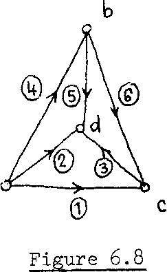
conditional adjustment. The configuration of the levelling network in question is illustrated again in Figure 6.8, for convenience.

From the above mentioned example we have: No. of observations, n = 6, No. of unknown parameters, u = 3.

Then df = 6 - 3 = 3, and we shall see that we can again formulate only 3 independent condition equations between the given observations.

By examining Figure 6.8, we see that there are к closed loops, namely: (a ~ с - d - a), (a-d-Ъ-а), (b - с - d - b) and (a - с - b - a).

This means that we can write k condition equations, one for each, closed loop. However, one can be deduced from the other 3, e.g. the last mentioned loop is the summation of the other three loops.

Let us ..for instance, choose the following three loops :

loop I=a-c-b-a>

loop 11= a-c-d-a>

loop III = a«d-b-a. These loops give the condition equations as follows

^(E1 ^{+ V}l⁾ " ⁽^6 ⁺ V " ⁽4 * V ⁼ °'

^1 ^{+ V}l^ ⁺ ^3 ⁺ V " ^2 ^{+ Y}2^ ⁼ °> (h₂ + v₂) - (h₅ + v₅) - (h^ + v^) = 0.

Then we get

^vi - v_k - v₆ + (5₁ - h_k - Eg) = 0 ,

^Vl - ^Y2 ^{+ V}3 ^{+ (5}1 " ^E2 ⁺ V ⁼ °> ^V2 " ^rk ~ ^v5 ^{+ (й}2 " \ ~ S^{) =} ° '

The above set of condition equations can be written in the matrix notation as

В V + ¥ = 0 , 3,6 6,1 ЗА

where:

	1	0	0	-1	0	-1
В	1	-1	1	0	0	0
3,6
	0	1	0	-1	-1	0

f = (V ^T2' ^YV V V V 1,6

and

¥ = 3,1

(h^ - h₂ 4 h^) ^(h₂ - \ - h₅)j

Substituting the observed quantities h\ , i = 1, 2, 6,

W = 3,1