Into the above vector we get 0.0

0.0 In metres .

-0.1

The weight matrix P of the observations is formulated as: (see example 6.17):

P = diag (0.25, 0.5, 0.5, 0.25, 0.5, 0.25) 6,6

and

P"¹ = diag (k, 2, 2, k, 2, k). 6,6

The normal equations for the correlates К are

M К = W 3,3 3,1 3,1

where

м =	В р"	-1 Т В =	12	k	к
3,3
			k	8	-2
			k	-2	8
inverting	I М we get:
		0.15	-0.1		-0.1
-1
М	=	-0.1	0.2		0.1
3,3
		-0.1	0.1		0.2

The solution for К is given Ъу

0.15 -0.1 -0.1 -0.1 0.2 0.1 -0.1 0.1 0.2

К = M~¹W = 3,1

	0.0		0.01
	0.0	=	-0.01
	-0.1 e		и -0.02

-1 т - P в к

The estimated residuals are computed from equation (б.Юб)

Г

V

6,1

m

0.00 0.02 0.02 -0.0U -0.0k

L o.ou _

and are again identical with the results of example 6.17, The adjusted observations will be.

	L = L +	V , i	• e.
		6.16		0.00
		12.57		0.02
ь		6.Hi		0.02
		1.09	T	-0.0U
		11.58		-0.0k
к		5.07	1	0.0k

6.16 12.59

6ЛЗ

1.05 11. 5^

5.11

In metres.

Finally, to compute the estimated elevations of points

b, c, and d, i.e. , H^ and H , we will use the given

elevation H and the adjusted observations h..

a l

For instance;

= H_a + h^ = 0.0 + 1.05 = 1.05 m,

H = H + h = 0.0 + 6.16 = 6.16 m, с a 1

H. = H + h_n = 0.0 + 12.59 = 12.59 m, d a 2

These are obviously identical with the corresponding results of the parametric adjustment.

Note again that when computing the estimates of the unknown parameters from the adjusted observations we can follow any route in computing them. They all lead to the same answer.

6.k.11 Variance-Covariance Matrix of the Conditional Adjustment Solution

The formula for the variance-covariance matrix of the adjusted

L

observations - the "result" of the conditional least squares adjustment -can be developed by applying the law of propagation of variance-covariance matrix (equation 6.15) on equation (6.113). In this equation, the matrices I,T,H are, obviously, fixed. Similarly, the vector С is considered as a vector of theoretically deduced, and therefore errorless, values, then will be zero. Hence, we get:

ч * <§> ч <§>^T

= (i - T) Zj. (I - T)^T

= Z- - IE- T^T - TZ-I + TZ-T^T. ir L L L

(6.115)

It is not difficult to see that both (IZ-T ) and (TZ-l) are square symmetric

L Jj

matrices, hence we can write:

Z; = Z- - 2TZ-I + TZ-T^T L L L L

= z₇ - tz- (21 - т ;.

(6.116)

Recalling, from equation 6.11U , that T = P"¹ [B^T(BP^b"¹")] and

2 -1

knowing that P = a Z- , i.e.

о Jj

2 —1

Z- = a P , then by substituting these quantities into equation (6.1l6)

Li О

we get:

z; = a ² p^_1 - a ² p"¹ [b^t(bp^_1b^t)^_1b] p^-1* L о о

к {21 - (p~¹[b^t(bp"¹b^t)"¹b]^t}

(6.ИТ)

Р —1 ф —1 ф —1 «Л

= о Р { I - 2[В (BP В ) В] Р +

+ В^Т (ВР"¹В^Т)"¹(ВР"¹В^Т) (ВР^_1В^Т)^_1 БР^-1}.

И"

м

и

-I

we get finally

Noting that

((bp~¹b^t)"¹)^t = (вр^-3^)"¹

? —1 ф 1 Ф 1 —1

Ел = а Р (I - В (BP В ) BP ) ♦

L о

(6.118)

Here, similar to the parametric adjustment, to obtain the estimated

^л 2 2

variance-covariance matrix we use a instead of а , where:

о о

^{л 2} V PV _ V PV ^ао df " г

(6.119)

and we end up with

z; = о ² (p^_1 - p"¹ b^t (BP^B¹)"¹ bp"¹) , (6.120)

L о

or,in an abbreviated form:

i: = а ² (I - Т)]?""^{1 6}) . (6-121)

L о

Analogous to the parametric adjustment, it also can be shown

that the estimate L assures the minimum trace of its variance-covariance

matrix E". Under the same assumptions as stated in section 6Л.8, the J_j

estimate L is also the most probable estimate of L.

Regarding the correlation between the adjusted observations

/Ч A

L, we can see that L will be uncorrelated if:(i) L is uncorrelated and (ii) the coefficient matrix В is orthogonal. If these two conditions are satisfied then T and P ^ will be diagonal matrices. On the other

л

hand, we can experience uncorrelated L even for some other general T and P.

Finally, we note that again the choice of the a priori variance factor a ^ does not influence the estimated E£ defined by equation (6Д21),

л

Example 6.22: Let us determine the var i anc е-соvari anc e matrix E" for the

L

conditional adjustment formulated in example 6.20. We have

ЛН - Eh.

_{v =} —¹ d. , i = 1, 2, 3,

¹ ?d. ¹

l l

and P = diag (~~, ~~).

3,3 1 2 ^a3

2 -1

Thus we get

а ₂ vV Cah-ZS,)

0. - . — i

Ed.

1 1

The required variance-covariance matrix is given by equation 6.121, i.e.

e; = a ² (i - T) P"¹.

L о

-1 T -1

First we compute T = P В M B. We recall from example

6.20 that M""¹ = 1/rd. , В = [1,1,1] 1,1 i ¹ 1,3

and P ¹ = diag (d , d , d ).

3,3 ■

Hence,

dl	0	0
0	d^ 2	0
0	0	d3

[ i—] [1, 1, 1] Zd,

and we obtain

^ _ 1

3,3 {i_±

2 ^d3

Further we get (i - T) p"¹

5 3

where a. = d, - -=-r~ i l Ed.

i = 1, 2, 3-

Finally we get

^{л л} р ««."1

Е Г ' = а (I - Т) Р

з,з^ь

_ 2

(ДН - ?^hi)

Ed. i l

⁴

3]

Example б»23: Let us determine the variance-covariance matrix for the conditionally adjusted levelling net of example 6.21. We have

V^T = [0.00, 0.02, 0.02, -0.04, -0.0^, 0.0k] 1,6

in metres,

g ₆ = diag [0.25, 0.5, 0.5, 0.25, 0.5, 0.25] 2

in m , and

r=df=n-u=6-3=3 Hence,

Am A

^л Ш . V PV 0.002 а * s —-—

о f r 3

V PV = 0.002 (unitless),

= 0.00067 (unitless),

The required matrix is computed again from equation L

6.121 as

z; = а ² (I - T) p""¹

L о

6,6

where

P^_1 = diag [k, 2, 2, 1», 2, h] 6,6

and T is computed from

T = 6,6

p^-1 (b^tm^-1b)

Hence _}

(в^тм^_1в) =

0.15 -0.1 0.1 -0.05 0 -0.05

-0.1 0.2 -0.1 -0.1 -0.1 0

0.1 -0.1 0.2 0 -0.1 0.1

-0.05 -0.1 0 0.15 0.1 0.05

0 -0.1 -0.1 0.1 0.2 -0.1

-0.05 0 0.1 0.05 -0.1 0.15

and: T = P^-1 (B^TM^-1B) = 6,6

0.6	-оЛ	O.k	-0.2	0	-0.2
-0.2	0Л	-0.2	-0.2	-0.2	0
0.2	-0.2	OA	0	-0.2	0.2
-0.2	-оЛ	0	0.6	O.k	0.2
0	-0.2	-0.2.	0.2.	оЛ	-0.2
-0.2	0	оЛ	0.2	-оЛ	0.6

Hence

(I - Т) Р"¹ =

1.6	-0.8	0.8	-0.8	0	-0.8
-0.8	1.2	-ОД	-0.8	-ОД	0
0.8	-ОД	1.2	0	-оД	0.8
-0.8	-0.8	0	1.6	0.8	0.8
0	-ОД	-ОД	0.8	1.2	-0.8
-0.8	0	0.8	0.8	-0.8	2Д

Finally we get

z; = a ² (I - T) P^_1 as L о

6,6

» 10

10.72	-5.36	5.36	-5.36	0	-5.36
-5.36	8.Oil	-2.68	-5.36	-2.68	0
5.36	-2.68	8.Oil	0	-2.68	5.36
-5.36	-5.36	0	10.72	5.36	5-36
0	-2.68	-2.68	5.36	8.0k	-5.З6
-5.36	0	5.36	5.36	-5.36	16.08

in metres squared.

-U 2

By dropping the scalar 10 we get the results in cm .

The comments stated at the end of section 6Л.9 regarding

^л 2 2

the value of a versus the assumed vialue of 1.0 for a о о

hold true here as well.

6.5 Exercise б

1. То determine the height h of a vail shown in the Figure, the

h orizontal distance I and the vertical angle 9 were observed and found to be:

= 12°37^f30^f\ with S" = 10" ^ ⁰

£ = 85.3U m, with S~ = 2 cm.

Required: Compute the statistical estimate for h along with its RMS.

2. To determine the distance P P = с, which cannot be measured directly

due to the existence of some obstacle as shown in the Figure, the

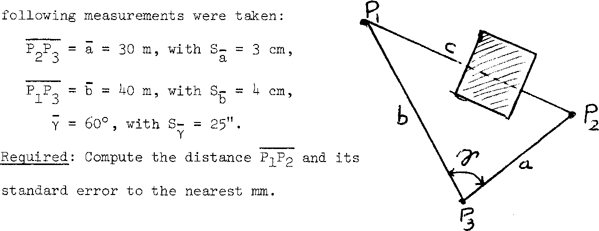
3. Determine the standard error of the estimated height h of the tower given in Problem number 9, Exercise k, section h.ll. Consider all the measured quantities, namely £, a, g and 0 to be uncorrelated.

k. From a point P_Q in the x-y coordinate system shown below, a distance d = 5637.8 m and an azimuth T = Н9.987З grads (100 grads = 90 degrees) to a second point P^ were measured. The relative error of cL is 1.2 • lO"^. The RMS of T is 0.08 centigrads (l grad = 100 centigrads).

Required: Compute the following:

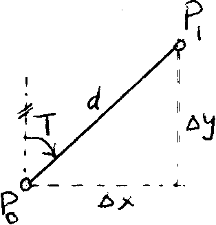
(i) The coordinate differences (Ax, Ay)

between points P and P_.

¹ о 1

(ii) The variance-covariance matrix , where X = (Дх, Ay), in m . 'iii) The RMS of Ax and Ay respectively, (iv) The correlation coefficient between Ax and Ay.

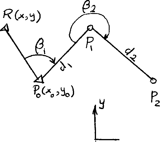
5. The shown traverse consists of two legs P^P^ and P^P^. The coordinates (x_q, у ) of the initial point P_q as well as the (x, y) coordinates of the reference mark R are considered to be error-free (errorless) , i.e. fixed quantities. The measured quantities are the horizontal angles and 3^

and the horizontal distances d^ and d^ respectively. The available data are:

x	= 100.0 m		У =	200	. 0 m ,
x о	= 150.0 m	»	Yo =	150	.0 m ,
h	= 75° ,	with	V	3"	Э
2	= 270° ,	with	%-	2"	5
h	= 100 m	and	d2 =	200	m.

The standard error of the observed distance is to be calculated according to the formula :

Sr(cm) = 1.0 •(cm) + d(m) . 10 d

Required: Compute the following:

(i) The estimated coordinates (x-^, y^) of point along with their

associated variance-covariance matrix Z/" ч .

(х_1э y_x)

(ii) The estimated coordinates (X2, y₂) °? point and their

variance-covariance matrix ^A _N.

U₂, y₂)

Note that the coordinates are required to the nearest щ and the variances and covariances are required in cm ²

(iii) Discuss the correlation among the estimated coordinates x ₉ y^, x₂ and j₂.

Having an intersection problem, as shown in the Figure _э i.e.

observing the two horizontal angles 3 and a from the two known stations

P^ (x-^j y^) and P^ (x^, у ) in order to determine the (x, у) coordinates

of an unknown station P. Given: the following data:

2

cm, ₅

cm

x = 200.0 m у = 500.0 m

k 1

-0.5

^{5 E(}*l> ^1^} \l 2

x = 5^-6. U m

, Z,- - ) =

S- = 3»

a

S- = 2^й

y₂ = 300.0 m ^^x2' ^y2 (-0.5 3

and S = 0 .

a = 90° 0 = 60°

Required: Compute the estimated (x, у) coordinates of the unknown

station P, in metres, and their associated variance-covariance matrix 2

Z, ч in cm (x, У)

Т. Consider problem number 1 of this exercise. Assume that the observed quantities I and 9 have got also non-random (systematic) errors of -1 cm and 5" respectively. Compute the expected total error in the derived height h in centimetres.

8. Determine the expected error in the sum of a hundred numbers in the following two cases:

(i) each individual number is to be rounded-off to three decimal places.

( ii) each individual number is to be truncated to three decimal places.

Then compare and comment on the results.

9* To determine the height h of a tower, the technique shown in the Figure'" was proposed, in which, a, g, 9 and a are the quantities to be measured. The approxi- mate values of these quantities were obtained from a preliminary investigation and found to be: a = 60° , g =30° ,

0 = k5° and a = 100 m.

h

Providing that the horizontal angles a and g are to be measured with a precision of 2" (i.e. S~ = = 2"), what are the required precisions in measuring both the horizontal distance a and the vertical angle 9

(i.e. S- and S-) such that their contributions to the standard error S,

а у

of the derived height h - which is specified not to be worse than 2.^5 сш - will be the same.

10. Assume that the horizontal angles in a triangulation network are to be measured using two theodolites , "I" and"II^м , of different quality. These two theodolites were tested by measuring one particular angle several times, from which it was found that the standard deviation

of one observation, i.e. the standard deviation of the sample,observed

with theodolite "I" was S = 1V5 and with theodolite "II"

^Ll

was S = 2^!.^?5. If it is specified that all the angles of the net-

²

work are required to have a standard deviation of the mean, i.e. S-, not worse than 07 5, how many times should we measure each angle when using theodolite number"l" and when using number "II"?

11. The following observations of the length of an iron bar in metres are made on a comparator:

3.28U, 3.302, 3.253, 3.273, 3.310, 3.321, 3.30*+, 3.295, 3.263, 3.270. Required: (i) the length of the bar (i.e. the mean) ; (ii) the RMS of one observation j (iii) the standard deviation of the mean.

12. The following table shows the means of the daily measurements of

the same distance I during a five day period, along with their

respective standard errors S~ .

i

Day	Mon.	Tues.	Wed.	Thurs.	Fri.
l± (m)	101.01	100.00	99-97	99.96	100.02
i	2	1	к	5	3

Required: Compute the weighted mean of the distance £, say £, along with its associated RMS, i.e. S j.

Given a gravimetric network, as shown in the figure below, determine the gravity values g^ and g^ at points P^ and P^ respectively_}

w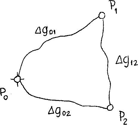 ith their variance-covariance matrix. The gravity

g_Q = 979832.12 mgal at the initial point P^ is known.

The following table gives the observed gravity differences with their signs , along with the time needed for each observation.

Station		Ag (mgal)	ДТ (hr)
From	' To
P 0		- 9.82	2.5
P2	po	-27.78	1.5
Pl	P2	+38 Л2	2.0

Assume that the observed differences Ag^fs are uncorrelated, and their variances are proportional to the corresponding time intervals AT.

¹ 4

length I. of each section.

Section	Station		h.	I. 1 (km)
No.	From	To	(m)
1		В	1.2U5.	1.0
2	A	pi	0.990	0.5
3	pi	P2	0.500	1.0
1+	P2	В	0.751	1.0
5	P3	в	1Л86	0.5
6	P3	P2	0.7^0	1.5

Note that the arrows in the given figure indicate the directions of

increasing elevations. The above observations are considered

2

uncorrelated with S~ proportional to

i

Required: Perform a parametric least squares adjustment of the above levelling net and find out the following:

(i) The estimated elevations H^, and of points P^ and P .

(ii) The adjusted values of the given six height differences.

^a2

(iii) The estimated variance-factor and compare it with the assumed₅

2

apriori variance factor S^; comment on the results.

(iv) The estimated variance-covariance matrix of X = (H ,H , H ).

X 1 <d j

15. Adjust the levelling net given in problem no. ih again by using the conditional method of adjustment. Replace the requirement no. iv by computing the estimated variance-covariance matrix of the adjusted height differences. Compare the results of the other three requirements with the corresponding results from the parametric adjustment.

l6. Two physical quantities Z and Y are assumed to satisfy the following linear model

Z = aY + g ₉

where a and g are constants to be determined. The observations Y^ and Z^ obtained from an experiment are given in the following table.

Y	1	3	k	6	8	9	11	11*
Z	1	2	k	h	5	7	8	9

Assume that the Y^fs are errorless, and the Z^? s were observed with equal precision.

Required: Determine a and g which provide the best fitting line between Z and Y, in the least squares sense.

17» Solve problem No. l6 again, but this time consider the Z^!s error­less , and the Y^!s with equal variances. Compare the results for a and 3 with the corresponding results from problem No. 16.

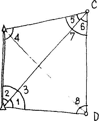
18. The given figure shows a triangulation network with fixed base AB = 2 km. The eight numbered angles in the Figure are all measured, each with a

different number n. of observations

i

as shown in the following table:

в

Angle Ко.	п. i	Mean	value	of the angle
1	2	82°	07'	09'.'50
2	2	28	22	17-70
3	5	110	29	25.02
к	3	125	53	33.67
5	2	25	kk	09.30
6	2	29	19	17-50
7	5	55	03	29.32
8	3	68	33	32.33

Assume that all the measurements were done with the same instrument and under similar circumstances. (Hint: the weight of each angle will be proportional to the corresponding number of repetitions n^). Required: (i) Neglecting the spherical excess in this network, compute the distance CD using the adjusted values of the observed angles.

(ii) Considering the fixed base AB to be errorless, find the estimated relative error of the estimated length CD.

The given figure shows a braced quadrilateral ABCD in a triangulation network, in which all the directions marked by arrowheads were measured with the same precision. _л

27 ^v26

32 >ИЗ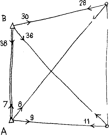

The base AB = 25 km is assumed errorless. The spherical excess e in the four formed triangles is computed apprоximately and given by:

ЛАВС, e = 3V126 ,

AABD, e = l^f.^!556 )

ACBD, e = 3V085 ,

AACD, e = 17515 . The results of the direction observations are summarized in the following table.

D

Occupied	Target	Direction	Observed Direction
Station	Station	No.
	В	7	00°	00'	00'.'00
A	С	8	91	30	30.35
	D	9	125	53	33.91
	С	30	00	00	00.00
В	D	36	28	22	17.26
	A	38	110	29	27.13
	D	26	00	00	00.00
С	A	27	29	19	17.52
	В	28	35	03	26.80
	A	11	00	00	00.00
D	В	12	35	07	. 29.00
	С	13	68	33	32.60

Required: (i) Perform a conditional adjustment and find out the adjusted values of the observed directions, along with their

estimated variance-covariance matrix .

L

(ii) Using Legendre^T s theorem for the spherical triangle _y i.e. by subtracting one third of the spherical excess from each adjusted angle and then solvirg the triangle as if it was a plane triangle compute the side CD from the known base AB and the adjusted directions. Then check the computed CD by following another route in its computation.

(iii) Compute the estimated relative error of the estimated length CD.

20. The given figure shows a triangulation network with two fixed (errorless) stations

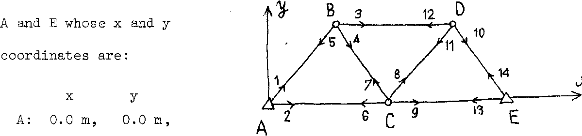
E: 200.0 m, 0.0 m.

The Ik marked directions (with arrowheads) were observed with the same precision. The results of the observations are tabulated below.

Occupied	Target	Direction	Observed		Directions
Station	Station	No.
л	В	1	00°	00	OO'.'O
ii	С	2	60	00	10.0
	D	3	00	00	00.0
В	С	h	60	00	05-0
	A	5	119	59	50.0
	A	6	00	00	00.0
с	В	1	59	59	55-0
	D	8	120	00	00.0
	e	9	180	00	05.0
	e	10	00	00	00.0
D	С	11	59	59	1+5.0
	В	12	119	59	55.0
	A	13	00	00	00.0
Ji	D	lU	60	00	15.0

Required: Prepare the input for a computer program performing a parametric least squares adjustment using the directions (not the angles) to estimate the unknown coordinates of points В, С and D by-providing the following:

(i) The number of unknown parameters and the number of degrees of freedom.

(ii) The non-linear mathematical model. (iii) The approximate values for the ,x, у coordinates of points B,C,D.

(iv) The linearized form of the mathematical model, i.e. V = AAX-AL, giving the symbolic elements of the vectors V and AX and the numerical values of the elements of the design matrix A and the vector AL.

(v) Construct the variance-covariance matrix E - of the ohser-vat ions assuming the standard errors in directions to equal 2".

APPENDIX I

Assumptions for and Derivation of the Gaussian PDF

The derivation of the Gaussian PDF presented here is. due to G.H.L. Hagen (l837)• The first formulation of the normal law, however,originates with De Moivre (1733).

(i) Let us assume that m independent physical causes are influ- encing the measurement. Let each cause contribute an elementary error either +A or -Л towards the overall error e. Any value of e can thus be expressed as a combination (there are n = 2^m such combinations) of m elementary errors + Д. We note first that the spaa of e is <-mA, mA>. Further, we realize that e can attain only a value of an integral multiple of A. It is not difficult to see that any two adjacent values of e differ by 2A since one is obtained from the other by replacing -A by +A and vice- versa. Dividing the range of e

Ra (e) = mA - (-mA) = 2mA by the step of e, i.e. 2A, we discover that e can attain any of the following m + 1 values

^ei ~ " ^Ш)^Д ' i = 0, 1, ... т. (1-1)

corresponding to particular distinguishable combinations of the m elementary errors.

(ii) Let us regard now the set D of all permissible values of e

the probability space of the random sample consisting of all the 2^m combinations e. Obviously, many of the 2^Ш combinations have the same values, because there are only m + 1 different values available. The counts, c^, of the individual values (see section 3.1.1) can be computed using the combined probability (see section 2.3):

_c_ _{= (}m_{} щ} m (m-l) (ш-2) ... ОачИ-l) ₌ J j/ n j. (l-2) ¹¹ i (i-1) (i-2) ... 1 j=m-i+l j=l

The actual probability of any value is then given by

P(._e ) ₌!l= ф/₂^ш , (1-3)

¹ n ¹

(see section 3.1.2).

(iii) The above formula describes the actual PDF of our sample e in the discrete probability space D. Since our ultimate aim is to derive the analytic expression for the "corresponding" (we shall see later what is meant by corresponding) continuous PDF, we want to be able to express P as a function of rather that i. The easiest way to do it is to use the finite differences.

Let us;.define

6P(e.) = P(e.) - P(e_iel)

and we get from equation (1-3)

_бр(_е.) = ф/2^Ш - (Д)/2^т

т

_^Ф-Фт3к^

= (^Ш)/2^т (1 - -4-г). 1 т-1+1

Obviously, the ratio 6Р (е^)/Р(е^) is then given by

6P(e_i)/P(e_i) = 1 - i/(m-i+l). On the other hand, i can Ъе expressed as a function of from equation (I-D

2i - m = e^/A

or 1

^{1 =} 2 ^^e±/^{A + m})•

Renoting <5e = 2A and substituting for i in equation (i-U) we obtain

6P(e) ₌ _ c/6_£ + m/2 P(e) m - e/бе- m/2 + 1

₌ 1 + m/2 - в/б£ - e/6e- m/2 1 + m/2 - e/6e

_ 1 - 2e/6e ₌ 2e - 6g

1 + m/2 - e/бе (l + m/2) 6e - e

(iv) The next step in the development is to convert the discrete PDF, P(e), to a continuous PDF, i.e. to derive the "corresponding" continuous PDF. The "corresponding" PDF is assumed to be the PDF of such a variable e which is defined the same way as the- discrete e in (i) with the exception that m is let to grow beyond all limits, i.e. m -> °°. By letting m grow we would obtain infinitely large values of e (see equation (i-l)). This would contradict our experience teaching us that the errors are always finite in value. Hence, we have to adopt another assumption and that is that as m grows to infinity, the absolute value of elementary error A grows to zero, making the product mA in equation (I-i) always finite.

Accepting these two assumptions we can write the finite difference equation as

6P(e) . 28 - бе

_{lim ——— = -» .lim ————————}

P<^e> (l+m/2) бе - e ^(l~⁵⁾

ш—> oo m ⁰⁰

6e -> 0 Se 0

which is nothing else hut an ordinary differential equation for the con­tinuous PDF P(e). It can thus he rewritten as

d P(e) 2e - de

P(e) (1 + m/2) de - e

To simplify the solution of this differential equation let us multiply

both the numerator and denominator of the right hand side by de and assume 2

that mde " is constant We further assume

2 2

de << ede << mde = С .

Then we can write

P " С/2 С

dP 2 ede k

ede . (1-6)

(v) We can now finally solve the differential equation. It is solvable by direct integration and we get

f— = - ede + const,

. k e² in P = - ~ — + const.

Denoting the integration constant by Лn К we finally obtain

P = К exp (~2e²/C). (i-T)

The question now arises whether we are free to regard both К and С as two independent parameters of the above PDF. We know that the basic equation for a PDF, i.e

/ °° P(e) de = 1 (1-8)

™.oo

has to be satisfied. Substituting for P into the basic equation we get

f P(e) de = / К exp (-2e²/C) de =

К / exp (-2e²/C) de = 1

and К = 1 / / exp (-2e²/C) de

Hence the answer is that К must not be regarded as an independent parameter. It is a function of С and can be evaluated by solving the integral above. We obtain

00

_{/ exp (-2e2/C) de = 2 / °° exp (-2e2/C) de = / — (1-9)}

m 0

and К ~ / . (1-10)

Стг

The Gaussian PDF can then be written as

P(e) = G (C;e) = exp (-2e²/C) (i-ll)

and we can see that it is a one-parametric PDF.

APPENDIX II - A

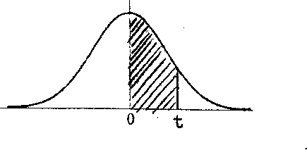
' ■* ORDINATES OF THE STANDARD NORMAL CURVE . Y = exp .(-, —) V2* 2		Y. j	N.
	° t

t	0	1	2	3	•■• 4	5	6	7	8	9
O.Q	.3989	.3989	.3989	.3988	.3986	.3984	.3982	.3980	.3977	.3973
од	„3970	.3965	.3961	.3956	.3951	.3945	.3939	.3932	.3925	.3918
0.2	.3910	.3902	.3894	.3885	.3876	.3867	.3857	.3847	.3836	.3825
0.3	.3814	.3S02	.3790	.377?	.3765	.3752	.3739	.3725	.3712	.3697
0,4	.3683	.3668	.3653	.3637	.3621	.3605	.3589	.3572	.3555	.3538
0.5	. .3521	.3503	.3485	.3467	.3448	.3429	.3410	.3391	.3372	.3352
0.6	.3332	.3312	.3292	.3271	.3251	.3230	.3209	.3187	.3166	.3144
0.7	.3123	.3101	.3079	.3056	.3034	.3011	.2989	.2966	.2943	.2920
0.8	.28.97	.2874	.2850	.2827	.2803	.2780	.2756	.2732	.2709	.2685
0.9	.2661	.2637	.2613	.2589	.2565	.2541	.2516	.2492	.2468	.2444
1.0	.2420	.2396	.2371	.2347	.2323	.2299	.2275	.2251	.2227	.2203
1.1	.2179	.2155	.2131	.2107	.2083	.2059	.2036	.2012	.1989	.1965
1.2	Л942	.1919	.1895	.1872	.1849	.1826	.1804	.1781	.1758	.1736
1.3	.1714	.1691	.1669	.1647	.1626	.1604	.1582	.1561	.1539	.1518
1.4	.1497	.1476	.1456	.1435	.1415	.1394	.1374	.1354	.1334	.1315
1.5	.1295	.1276	.1257	.1238	.1219	.1200	.1182	.1163	.1145	.1127
1.6	.1109	.1092	.1074	.1057	.1040	.1023	.1006	.0989	.0973	.0957
1.7	.0940	.0925	.0909	.0893	.0878	.0863	.0848	.0833	.0818	.0804
1.8	.0790	.0775	.0761	' .0748	.0734	.0721	.0707	.0694	.0681	.0669
1.9	.0658 •	.0644	.0632	.0620	.0608	.0596	.0584	.0573	.0562	.0551
2.0	.0540	.0529	.0519	.0508	.0498	.0488	.0478	.0468	.0459	.0449
2.1	.0440	.0431	.0422	.0413	.0404	.0396	.0387	.0379	.0371	,0363
2.2	.0355	.0347	.0339	.0332	.0325	.0317	.0310	.0303	.0297	.0290
2.3	.0283	.0277	.0270	.0264	.0258	.0252	.0246	.0241	.0235	.0229
2.4	.0224	.0219	.0213	.0208	.0203	.0198	.0194	.0189	.0184	.0180
2.5	.0175	.0171	.0167	.0163	.0158	.0154	.0151	.0147	.0143	.0139
2.6	.0136	.0132	.0129	.0126	.0122	.0119	.0116	.0113	.0110	.0107
2.7	.0104	.0101	.0099	.0096	.0093	.0091	.0088.	.0086	.0084	.0081
2.8	.0079	.0077	.0075	.0073	.0071	.0069	.0067	.0065	.0063	.0061
2.9	.0060	.0058	.0056	.0055	.0053	.0051	.0050	.0048	.0047	.0046
3.0	.0044	.0043	.0042	.0040	.0039	.0038	.0037	.0036	.0035	.0034
3.1	.0033	.0032	.0031	.0030	.0029	.0028	.0027	.0026	.0025	.0025
. 3.2	.0024	.0023	.0022	.0022	.0021	.0020	.0020	.0019	.0018	.0018
3.3	.0017	.0017	.0016	.0016	.0015	.0015	.0014	.0014	.0013	.0013
3.4	.0012	.0012	.0012	.0011	.0011	.0010	.0010	.0010	.0009	.0009
3.5	.0009	.0008	.0008	.0008	.0008	.0007	.0007	.0007	.0007	.0006
3.6	.0006	.0006	.0006	.0005	.0005	.0005	.0005	.0005	.0005	.0004
3.7	.0004	.0004	.0004	.0004	.0004	.0004	.0003	.0003	.0003	.0003
3.8	.0003	.0003	.0003	.0003	.0003	.0002	.0002	.0002	.0002	.0002
3.9	.0002	.0002	.0002	.0002	.0002	.0002	.0002	.0002	.0001	.0001

239

APPENDIX II-B

t	0	1	2	3	4	5	6	7	8	9
0.0	.5000	.5040	.5080	.5120	.5160	.5199	.5239	.5279	.5319	.5359
0.1	.5398	.5438	.5478	.5517	.5557	.5596	.5636	.5675	.5714	.5754
0.2	.5793	.5832	.5871	.5910	.5948	.5987	.6026	.6064	.6103	.6141
0.3	.6179	.6217	.6255	.6293	.6331	.6368	.6406	.6443	.6480	.6517
0.4	.6554	,6591	.6628	.6664	.6700	.6736	.6772	.6808	.6844	.6879
0.5	.6915	.6950	.6985	.7019	.7054	.7088	.7123	.7157	.7190	.7224
0.6	.7258	.7291	.7324	.7357	.7389	.7422	.7454	.7486	.7518	.7549
0.7	.7580	.7612	.7642	.7673	.7704	.7734	.7764	.7794	.7823	.7852
0.8	.7881	.7910	.7939	.7967	.7996	.8023	.8051	.8078	.8106	.8133
0,9	.8159	.8186	.8212	.8238	.8264	.8289	.8315	.8340	.8365	.8389
1.0	.8413	.8438	.8461	.8485	.8508	.8531	.8554	.8577	.8599	.8621
1.1	.8643	.8665	.8686	.8708	.8729	.8749	.8770	.8790	.8810	.8830
1.2	.8849	.8869	.8888	.8907	.8925	.8944	.8962	.8980	.8997	.9015
1.3	,9032	.9049	.9066	.9082	.9099	.9115	.9131	.9147	.9162	.9177
Г.4	.9192	.9207	.9222	.9236	.9251	.9265	.9279	.9292	.9306	.9319
1.5	.9332	.9345	.9357	.9370	.9382	.9394	.9406	.9418	.9429	.9441
1.6	.9452	.9463	.9474	.9484	.9495	.9505	.9515	.9525	.9535	.9545
1.7	.9554	.9564	.9573	.9582	.9591	.9599	.9608	.9616	Л625	.9633
1.8	.9641	.9649	.9656	.9664	.9671	.9678	.9686	.9693	.9699	.9706
1.9	.9713	.9719	.9726	.9732	.9738	.9744	.9750	.9756	.9761	.9767
2.0	. .9772	.9778	.9783	.9788	.9793	.9798	.9803	.9808	.9812	.9817
2.1	.9821	.9826	.9830	.9834	.9838	.9842	.9846	.9850	.9854	.9857
2.2	.9861	.9864	.9868	.9871	.9875	.9878	.9881	.9884	.9887	.9890
2.3	.9893	.9896	.9898	.9901	.9904	.9906	.9909	.9911	.9913	.9916
2.4	.9918	.9920	.9922	.9925	.9927	.9929	.9931	.9932	.9934	.9936
2.5	.9938	.9940	.9941	.9943	.9945	.9946	.9948	.9949	.9951	.9952
2.6	.9953	.9955	.9956	.9957	.9959	.9960	.9961	.9962	.9963	.9964
2.7	.9965	.9966	.9967	.9968	.9969	.9970	.9971	.9972	.'9973	.9974
2.8	.9974	.9975	.9976	.9977	.9977	.9978	.9979	.9979	.9980	.9981
2.9	.9981	.9982	.9982	.9983	.9984	.9984	.9985	.9985	.9986	.9986
3.0 ,	.9987	.9987	.9987	.9988	.9988	.9989	.9989	.9989	.9990	.9990
3.1	.9990	.9991	.9991	.9991	.9992	.9992	.9992	.9992	.9993	.9993
3.2	.9993	.9993	.9994	.9994	.9994	.9994	.9994	.9995	.9995	.9995
3.3	.9995	.9995	.9995	.9996	.9996	.9996	.9996	.9996	.9996	.9997
3.4	.9997	.9997	.9997	.9997	.9997	.9997	.9997	.9997	.9997	.9998
3.5	.9998	-.9998	.9998	.9998	.9998	.9998	.9998	.9998	.9998	.9998
3.6	.9998	.9998	.9999	.9999	.9999	.9999	.9999	.9999	.9999	.9999
3.7	.9999	.9999	.9999	.9999	.9999	.9999	.9999	.9999	.9999	.9999
3.8	.9999	.9999	.9999	.9999	.9999	.9999	.9999	.9999	.9999	.9999
3.9	1.0000	1.0000	1.0000	1.0000	1.0000	1.0000	1.0000	1.0000	1.0000	1.0000

APPENDIX II - С