In order to be able to use the tables of the standard normal

PDF and CDF for computations concerning a given normal random variable

X, we first have to standardize X, I.E. To transform X to t using

equation (^-13), then enter these tables with t. Thus, if we want,

for instance, to determine the probability P(x £ x ) we have to write:

x-y x -y

P(x < x_Q) = l-V^ ) . (^-19)

X X

This is identical to the probability P(t £ t ) that can be obtained from the standard normal tables.

Example k.2

0 04

Figure k.k - i

Suppose that the height h of a student

Is a normally distributed random

variable with mean y, = 66 inches and

h

standard deviation cr, = 5 inches. Find

h

the approximate number К out of 1000 students h inches tall: (i) h £ 68 inches (Figure U.U-i) * (ii) h £ 6l inches (Figure k.h^ii)}

* In most of the computer languages, this error function, erf (t) is a built-in function. Hence, it can be called as any library subroutine and evaluated more precisely than using the corresponding tables.

-1.0 о

Figure b.U-ii

-0.34 0 0.8

Figure iv

(iii) h _> Tk.6 inches (Figure k. ■

	1
IS A M

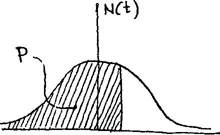
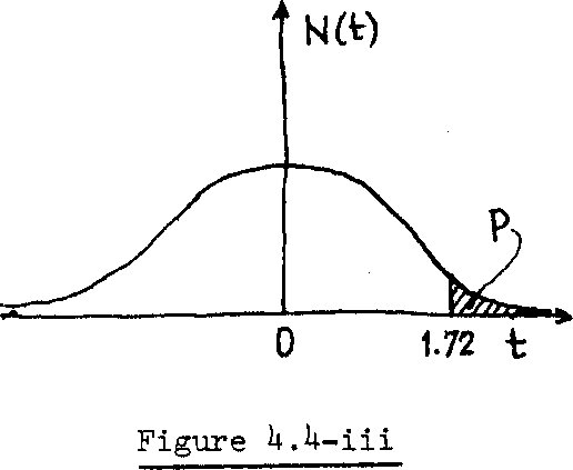
(iv) [6k.3 <. h <_ 70] inches (Figure U.U-iv), Solution: We are going to use the Table in Appendix II-B.

(i) P(h < 68) = P(t )

= P(t <. 0.U0) = 0.655*1 .

-t ' Hence, K_± = (0.655*0(1000) = 655 students, (ii) P(h 1 61) - P(t <_ii=66 _}

= P(t 1 -1) = 1-P(t <_ 1)

= 1. - 0.8U13 = 0.1587 . Hence, K₂ = (0.1587)(lOOO) = 159 students . (iii) P(h > 7b.6) = P(t > T^6-66 )

= P(t >_ 1.72)

= 1. - P(t <_ 1.72)

= 1. - 0.9573 = 0pU27 .

Hence, K_ = (0.0^27)(1000) = U3 students.

(iv) P(6U.3 1 h <_ 70) =

, p (бЬ.3-66 < _t <12=бб _}

= P (-0.3k < t < 0.80) = P(t £ 0.80) - P(t <. -0.3^)

= p(t 1 0.80) - (l-p(t <. 0.3k) = 0.7881 - [1-0.6331] = 0.7881 - 0.3669 = 0Д212 ,

Hence Кц = (0.U212)(1000) = U21 students.

Example 4.3

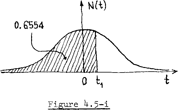
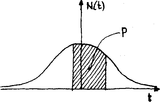
For the normal random variable h given in example 4.2, determine the student^f s height H such that: (i) P(h <, H ) = 0.6554 (Figure U.5-i) ;

(ii) P (h >, H₂) = 0.25 (Figure U-5-ii); (iii) P (h £ H ) = 0.20 (Figure 4-5-iii);

(iv) P(H₄£ h<H ) = 0.95,

where = y^-K and = y^+K. (Figure 4,5-iv) Solution: Again in this example, we are going to use the standard normal CDF table given in Appendix II-B. (i) P(h ± H ) = P(t ± t_±) = 0.655^ . From the above mentioned table, we get t = 0.4, that corresponds to probability P = 0.6554. But we know

H₁-u_h

that t_n = — •

^{1 a}h

From example 4-2 we have y^ = 66 inches

and = 5 inches. Hence, V-66

*1 ⁼ 5 " ⁼

from which we get

H - 66 = 5(0.4) = 2,

i.e.

H^ = 66 + 2 = 68 inches, which is identical to the first case in example 4.2; however_;what we are doing here is nothing else but the inverse solution.

юз

(ii) P(h >. H ) = P(t >. t ) - 0.25. But:

P(t >_ t₂)= 1-P (t £ t₂) = 0.25, and we get

P(t <_ t ) .= 1 - 0.25 = 0.75. By interpolation in the above mentioned table we get \, = 0.675 which corresponds to P = 0.75* Hence,

i.e. H₂ =66+5 (0.675)

= 66 + 3.375 = 69.375 inches .

(iii) P(h £ H₃) = P(t £ t₃) = 0.20 • By examining the above mentioned table we discover that the smallest probabil- ity reading is 0. 50, since it considers only the positive values of t, Therefore we have to write:

P(t 1 t₃) = 1 - P(t <r*₃) = 0.20,

and we get

P(t <?t^) = 1 - 0.20 = 0.80.

By interpolation in the above mentioned

table we get: (-t₃) = 0.81+2, which

corresponds to P = 0.80. Then we have: H -66

_{t =} — - -0.8U2

and, H₀ = 66-5(0.8U2)

3 5

^l3

= 66-U,210 =,6l.79 inches.

(iv) Р(Н^ <h£H₅)

₌ p₍_A_ii < _t < \

= < t < ^- )

= ^р(-*₀ <t£t ) = 0.95:

where t = — = — о a_{h 5}

The above statement means that:

^p(^t 1 *₀) - ^p("^t 1г*₀) ⁼ 0.95.

However, from the symmetry of the. normal PDF we get:

p(t > t_o) = P(t <.-t_Q) = ^1> " = 0.

and we get:

P(t £ t ) = 0.95 + 0.025 = 0.975, or P(t <_ t ) = 1. - 0.025 = 0.975. From the above mentioned table we get: t = I.965 which corresponds to P = 0.975э and we have: t_Q-f-1.96,

i.e. К = 5(1.96) = 9.80. Consequently H^ = |i_h-K = 66-9*B0 = 56.2 inches and

H₅ = y_h+K = 66 + 9.80 = 75.8 Inches.

can write:

P(-a < e < a ) = P(

Example k.k:

	i	i

Let us solve example 4.1 again by using the standard normal CDF tables. Recall that it was required to comput P(~a < e < a ), where e has a Gaussian PDF (i.e. its у = 0). We

-a -y . a -y

^{£ — — £}

a ~*0 , a

£ ■ ■ < t <

£ £ _{<t <} £

0

= P(

- — a

£ £

= P(-l £ t £ l) , see Figure 4.6.

Further we can write:

^p(-¹ <t < 1) = 2P(0 £ t £ 1).

From the table given in Appendix II-C

we get:

P(0 < t < 1) = 0.3413-Hence ₅

P(-a_P < £ < a ) = 2(0.3413)

= 0.6826 = 0.683, which is the same result as obtained in example 4.1.

U•T Basic Hypothesis (Postulate) of the Theory of Errors,

Testing

We have left the random sample of observations L behind in section k.2 while we developed the analytic formulae for the PDF*s mostly used in the error theory. Let us get back to it and state the following basic postulate of the error-theory. A finite sequence of observations L representing the same physical quantity is declared a random sample with parent random variable distributed according to the normal PDF Ж(у^_э cr^; a). Other PDF^T s are used rather seldom. The validity of this hypothesis may or may not be tested, on which topic we shall not elaborate here.

The mean of the sample L is said to approximate (the word estimate is often used in this context) the mean у of the parent PDF,

JO

2

i. e. N(y^3 a ^; Z). Also, the variance of the sample L is said to estimate the variance a| of the parent PDF.

Considering the original sample

L = u ) = u'+e ) , i = 1, 2, .. . , n,

we get:

n

^ML

- Y, £. = - /z, (£'+£.) = - (nA¹) + - e . = ' A¹ + M . (U-20) ⁿi=l ^{1 n 1=1} in n 1=1 1 e

Since the random errors e^T s are postulated to have a parent Gaussian PDF N(0₅ a_£; e )> which implies that = 0, then we should expect that M 0 and we can write equation (U-20) as:

e

M_L = = y_{£ 9} (U-21)

ют

keeping in mind that Ъу the unknown value l^} we mean the unknown mean

у of the parent PDF of I.

We say that the mean M of the sample L-

approximates (estimates) the value of the mean y^ of the parent PDF of £. Similarly₅ we get

2 1

Sf = - Л L n i=

n n m

l, (A.-JL Г = ¹ .I₁U.-(A^,+ M )] ^г = i lie. - M ) - S .=1 l V n 1=1 i e ^m--i=l ^{1 £ c}

The above result indicates that the variance S^ of the sample L is

2

identical to the variance S^ of its corresponding sample of random errors

2

£. This is actually why S is sometimes called the mean square error of

-Li ' ' '

the sample, and is abbreviated by MSE. Also, S_L is known as the root mean square error of the sample , and is abbreviated by RMS, According to the basic hypothesis of the error-theory we can write equation (4-22) as :

(b-23)

which states that S_T estimates the variance о of the parent PDF of

П

Example 4.3

Assume that the sample L = (2, 7₅ 6, 4,

2,7, 4, 8₅ 6, 4) is postulated to be

normally distributed. Let us transform

this sample in such a way that the transformed

sample will have:

(i) Gaussian distribution '»

(ii) Standard normal distribution.

Solution: First we compute the mean

2

and the variance S of the given sample as follows:

i ¹⁰ i

^M_T ^e io ill ^£i⁼Io-⁽⁵⁰⁾ = ⁵'

According to the basic postulate of the error-theory we can say that:

= ^ = 5 and _V a_£ = S_L = 2,

where у ^ and c^ are respectively the mean and the standard deviation of the parent normal PDF N (у , ; l) assumed for the given sample. The parameters

у ^ and о^ will be used for the required transformations as follows:

(i) The Gaussian distribution G(c_£; e), where ^G_£ ~ ^a£ ⁼ 2 _э has an argument e obtained from equation (^-10) as:

V^^r^' i - 2, ...,io.

Hence the transformed sample that has a Gaussian PDF is:

z = (e^, i = 1, 2, ... , 10 i.e.

- (-3, 2, 1, -1₉ -3, 2, -1, 3, 1, -1).

(ii) The standard normal distribution N(t), has an argument t obtained from equation (4-13) as:

*i ^e~^^s V-'¹ -^x'^{2 io}-

Hence, the transformed sample that has

a standard normal PDF is T = (t^)₅

i = 1, 2, . . . , 10 ₅ i.e.:

T = (-1.5, 1, 0.5, -0.5, -1.5, 1, -0.5,

1.5, 0.5, -0.5).

4.8 Residuals, Corrections and Discrepencies

As we have seen, we are not able to compute the unknown value I 'or y^. All we can get is an estimate 1 for it from the following equation

b^^'+M^ £^f+ e, *) (4-24)

and hope that e , in accordinace with the basic postulate of the error-theory, will really go to zero.

The residual r. is defined as the difference between the :— i

* From now on, we shall use the symbol I for the mean of the sample L. The "bar" above the symbol will indicate the sample mean to make the notation simpler.

observation £^ and the sample mean I, i.e.

(it.25)

Residuals with inverted signs are usually called corrections. It should be noted that a residual, as defined above, is a uniquely determined value and not a variable. The observed value SL is fixed and so is the mean £ for the particular sample. In other words, for a given sample, the residuals can be computed in one way only. Note that the differences (£_^ - £) = r^ are called residuals and not errors, because errors are defined as = (£^- y^) and y^ may be different from £.

In practice, one often hears talks about "minimized residuals", "variable residuals" etc. which are not strictly correct. If one wants to regard the "residuals as variables" the problem has to be stated differ­ently. The difference v^ between the observed value £^ and any arbitrarily assumed (or computed) value £°, i.e.

v. = £. - £°, i = 1, 2, . . ., n

l l

(U.26)

should be called discrepency, or misclosure, to distinguish it from the . residual. These discrepencies are obviously linear functions of £°jtheir values vary with the choice of £°. Hence one can talk about "minimization of discrepencies", "variation of discrepencies" etc. Evidently, residuals and discrepencies are very often mixed up in practice.

At this point it is worthwhile to mention yet another pair of

2

formulae for computing the sample mean £ and the sample variance S . Such

L

simplified formulae facilitate the computations especially for large samples

Ill

whose elements have large numerical values. The development of these formulae is done analogically to the formulation of equations (4.20), (4.22), (4.25) and (4.26). Here we state only the results, and the elaboration is left to the student.

C.2T)

I = £° + v ,

and

l=l

where: 1° is an arbitrarily cj^sen value, usually close to I_;

- 1 ⁿ

v = j Z v. , (4.29)

i=l

v.= £. - £° l l

and

r_± = l_± - I = v_i - v. (4.30)

Example 4.6: The second column of the following table is a sample of 10

observations of the same distance. It is required to compute

the sample mean and variance using the simplified formulae given in this section.

We take £° = 972.0 m,

1 ¹⁰ 1

v = ~q 'I v_± = (10.50) = 1.05 m,

i=l

X _s lo + у = 972.0 + 1.05 = 973.05 m,

MSE = ^Sl = lo ^{1 r}i^{2 s} 10 ^fo •^{5730) =} °'⁰⁵¹³' ^m2 i=l

and RMS = S_L = 0.24 m.

n

One of the checks on the computations is that Z r. = 0,

i=l ¹

see the fourth column of the given table.

Г""1 No.		; ■ ■ .v = Q _ 0°	r =1.-1	r.2 . 1014' (m )
	(m)	1 1 (m)	l 1 = V. - V 1
1	972.89	0.89	-0.16	256
2	973.1+6	1.1*6	0Л1	1681
3	973.ok	1.0k	-0.01	1
k	972.73	0.73	-О.32	1021+
5	972.63	0.63	-0.1+2	176b
6	973.01	1.01	-0.0k	16
7	973.22	1.22	0.17	289
8	973.10	1.10	0.05	, 25
9	, 973.30	1.30	0.25	625
10	973.12	1.12	0.07	1+9
	\ -i 1	10.50 * , .... _	-0.95 +0.95 = 0.00	5730

h.9 Other Possibilities Eegarding the Postulated PDF

The normal PDF (or its relatives) are by no means the only bell-shaped PDF¹s that can be postulated. Under different assumptions, one can derive a whole multitude of bell-shaped curves. Generally, they would contain more than two parameters which is an advantage from the point of view of fitting them to any experimental PDF. In other words the additional parameters provide more flexibility. On the other hand, the computations

-with such PDF's are more troublesome. In this context let us just mention that some recent attempts have been made to design a family of PDF¹ s that are more peaked than the normal PDF in the middle. Such PDF^fs are called "Leptokurtic"• This more pronounced peakedness is a feature that quite a few scholars claim to have spotted in the majority of observational samples. We shall have to wait for any definite word in this domain for some time.

Hence, the normal is still the most popular PDF and likely to remain so because it is relatively simple and contains the least possible number of parameters - the mean and the standard deviation.