4.10 Other Measures of Dispersion

So far, we have dealt with two measures of dispersion of a sample namely: The root mean square error (RMS) mentioned in section 4.7* and the range (Ra) mentioned in section 3-1.5- Besides the RMS and the range of a sample the following measures of dispersion (spread) are often used.

The average or mean error a of the sample l is defined as

Ill*

which is the mean of the absolute values of the residuals.

The most probable error p^, of the sample L, is defined as the

error for which:

P(|_r| < p ) = _P(|_r| > p ) _я o,50 в e

(U.31)

which means that there is '50$ probability that the residual is smaller and 5Q% probability that the residu&l is larger than p_e.

The most probable error of a random sample can be computed by constructing

the CDF of the corresponding absolute values of the sample residuals, and

take the value of r which corresponds to the CDF = 0.5 as the value of p^ .

Both a and p can be defined for the continuous distributions as e . e

well. For instance, by considering the normal PDF, N(^,0^; x), we can write:

00

a = / |x| ф (x) dx

⁰⁰ (х-м )²

₌ / |_x| _exp (_.-_£. у ах . (k.33)

a /( 2тг ) -оо 2a

X X

Similarly for p , by taking the symmetry of the normal curve into account,

we can write:

1 (У -P.) ^(x-Pv⁾²

Vm^Tj ^f exp (-—^) too 0.25 (U.3U)

_{p(* < \ - pe) = V\ - pe} *}

x -⁰⁰ 2a

x

and

P(x < u_x + p_e) = *_N(ji_x + p_e) = 0.75 (U.35)'

where 4* is the normal CDF. N

It can Ъе shown for the normal PDF N(u , a ;x) that "a " "a and "p "

-XX X с e

are related to each other by the following approximate relation:

a = 1.25 а = 1.5 p ,

x e ^e

or

(h.36)

a : а x e

i.o ;' o.8o I о.бт .

The relative or proportional error r^ , of the sample L, is defined

as the ratio between the sample RMS and the sample mean, i.e.

r = S_T I %. (4.37)

e L

In practice, the relative error is usually used "to describe the uncertainty of the result, i.e. the sample mean. In that case, the relative error is defined as:

(U.38)

r = S / I

⁶ ,7

where S is the standard deviation of the mean I and will be derived later

I

in Chapter 6.. In this respect, one often hears expressions like "propor­tional accuracy 3 ppm (parts per million)", which simply means that the relative error is 3/10^ = 3 * 10 ^. It should be noted that unlike the other measures of dispersion, the relative error is unitless.

The idea of the confidence intervals is based on the assumption of normality of the sample, i.e. the postulated parent normal PDF (N (£, S ;£)) for the random sample L. It is very common to represent the

sample L by its mean 1 and its standard deviation S as

L

¹1^S_L]

or

[I- - S < A < 5 + S ] ,

Й.39)

and refer to it as the "68% confidence interval" of I. This is based on

the fact that the probability P(y - a < I < у + о A is approximately 0.68 for

X/ X/ —¹ — Xj Xj

the normal PDF (see section 4.5).

Similarly, one can talk about the "95% confidence interval", the "99% confidence interval", etc. In general, the confidence interval of I is expressed as:

[I + К S ] (4.4o)

where К is determined in such a way as to make

P(y_£ - Ka_£ < I < y_£+Ka_£)equal to 0.95, 0.99, etc. The values (I - KS_T) and (I + KS_T) are called the lower and the

L Li

upper confidence limits.

Example 4.7'- Let us compute the average error_дthe relative error and the 95% confidence interval for the sample of observations L given in example 4.6.

The average error is computed using equation (4.31) and the

fourth column of the given table in example 4.6 as:

10 _±

_{a я} _ _z |_r, j = — (1.90) = 0-19 m .

^e io i=i ^{1 10}

The relative error of the sample is computed from equation (4.37) and the results obtained in example 4.6 as:

^re ^{= S}L ^{1 1} " 9тШ = .^-Effi •

The 95% confidence interval of I is

[I - К S <£<jE + KS_T] . L — — Li

where the number К is computed so that

P(y_£ - Ka_£ < I < H_A+Ka_£) = 0.95 -

This is identical to the probability P(-K < t < K) obtained from the standard normal tables (see example 4.3, the last case). Hence we can write:

Р(-К < t < К) = P(t < К) - P(t < -К) = 0.95

from which we get

P(t < K) = 0.975. Using the table for the standard normal variable of Appendix II - В we get:

К = I.96 ,

(in practice К = 2 is usually used for the 95% confidence interval.) The 95% confidence interval of & then becomes

[973.05 - 1.96 (0.2*0 < £ < 973.05 + 1.96(6.210 ]_; that is:

[972.58 < £ < 973.52] m

or

[973.05 + 0Л7] m.

A H(h)

x

Example h.8: Given a random variable x assumed to have a normal distri­bution N (35 э 1*; x) _э compute the most probable error. From the assumed PDF we have: у =35 and a = k.

x

The most probable error p^ is computed so that

P(y - p < x < у + p ) = x e - - x ^re

= P(-t < t < t ) = 0.'5©₉ (Figure U.7a) p - - p

P p e e where t = — = 1— . pa k ■^r x

The above probability statement can be rewritten as' (equation

(u.35)):

P(x < ja + p ) = P(t < t ) = 0.75 - x ¹ e - P

(Figure U.Tb '

Ф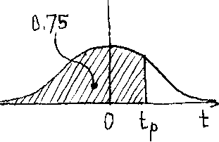 К/Ш From the table in Appendix II - B, we obtain t = 0.675

P

p = k t = Ij. (0.675) = 2.7 . e p —^L

corresponding to P = 0.75- Hence,

Figure к. 7b

Note that in the second case of example ^.3, the value 3.375 is nothing else but the most probable error of the given random variable h.

4.11 Exercise 4

1. Prove that the Gaussian PDF given by equation (U.1+) ₅ has two points of inflection at abscissas + /С/2.

2. For the Gaussian PDF given by equation (H.8), determine approximately the probabilities: P(-2a < e < 2a ) and P(-3a < e < 3a )

£ - - £ £ - - £

by integrating the PDF, then check your results by using the standard normal tables.

3. Prove by direct evaluation that the standard normal PDF has a standard deviation equals to one.

k. Show that the standard deviation a, average error a^ and the most pro­bable error p^ of the normal PDF satisfy the following approximate relations:

a : a ; p = 1.0 ; 0.80 : 0.67.

5. Determine: the average error, the most probable error, the relative error and the 90% confidence interval of the random sample given in the second problem of exercise 3₅ section 3.4.

6. Assume that the sample H = (-5, -4, -3, -2, »1, 0, 1, 2, 3, 4, 5) is hypothesized (postulated) to have a Gaussian distribution. Transform this sample so that the transformed (new) sample will have:

(i) Normal distribution with mean equal 10.

(ii) Standard normal distribution.

7. Given a random variable x distributed as N (25 , 10; x), determine the following probabilities:

(i) P(x < 28.5) %

(ii) P(x < 22.5) %

(iii) P(x > 27.5) ;

(iv) P(l6.75 < x < 23.82)j

(v) P (|x-25| < 1.25).

8. For the random variable in the previous problem, determine the values Z. such that

i

(i) P(x < Z_x) = 0.65, (ii) P(x < Z ) = 0.33 > (v) P(|x-25| > Z ) = 0.50.

(ii) P(x > Z₂) = 0.025 ; (iv) P(|x-25| < Z_u) = 0.33 ,

Л

The above figure shows a surveying technique to determine the height h of a tower CD, which cannot be measured directly. The observed quantiti are:

£ = the horizontal distance AB > a ,8 = the horizontal angles at A and В _; 9 = the vertical angle of D at В .

The field results of these observations are given in the following table

Average temperature during the observations time was T = 20° F. The following information was given to the observer: (iy The micrometer of the vertical circle of the used theodolite was not adjusted to read 001 00" when the corresponding bubble axis is horizontal; it reads - (00f 30")• (ii) The nominal length of the used tape is 20 m at the calibration temper­ature Tq = 60° F, and the coefficient of expansion of the tape material is у = 5 . 10~5 / 1° F . Field Observations
Mm)	a		3	e
1А5.6З	65° 32'	03"	37° 13' 08"	k2° 53'	15"
• 55	32	0U	13 11	52	30
• 59	31	59	13 10	53	00
.65	32	01	13 13	51	00
• 58	31	58	13 06	52	15
			13 12	52	U5
				51	15-
				53	00
				51
				.52	15
*

Required

(i) Compute the estimated values for the quantities £, a, g and 9 *

(ii) For each of the above observed quantities compute its standard de- viation and its average error.

(iii) Compare the precision of these observed quantities (by comparing the respective relative errors)•

(iv) Assume that each of these observed quantities has a postulated normal parent PDF, construct the 95% confidence interval for each quantity.

(v) Compute the estimated value of the tower^Ts height h to the nearest centimeter с

12 3