

5. Least-squares principle
5.1 The Sample Mean as "The Least Squares Estimator"
One may now ask oneself a hypothetical question: given the sample L = (, i = 1, 2, . .. , n, what is the value £° that makes the summation of the squares of the discrepancies
Vi = £i " £° 5 1 = 1э 2э * * * ' Пэ (5-1)
the smallest (i.e. minimum)?
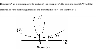
The above question may he stated more precisely as follows: Defining a "new variance" S*2 as
S*2 = - Z U.-£°)2=~ Z v2 , (5-2)
n i==1 i n 1=1 1
find the value £° that is going to give us the smallest (minimum)
2
value of S* .
Obviously, such a question can be answered mathemat i с ally. From equation (5-2), we notice that S*2 is a function of £°, which is the only free variable here, and can be written as
S*2 = S*2U°) . (5-3)
We know that:
3S*2
min [S* (£°) ] implies that = 0 .
£°eR Э£°
Hence, by differentiating equation (5-2) with respect to 1° and equa*-ting it to zero, we get:
n i=1 L3£o x
= — E [2(4.-A°)(-l)] =~ U.-4°) = 0 , n i=1 l n 1=1 l '
that is:
E (1.-1°) = 0
i=l i
The above equation can be rewritten as:
n n
I £. = 2 1° = n£° , i=l 1 i=l
which yields
1° = ^ ? 4. = I (5-4)
П 1=1 1
The result (5-4) is nothing else hut the "sample mean" 1 again. In other words, the mean of the sample is the value that minimizes the sum of the squares of the discrepancies making them equal to the residuals, (see section 4.8).
This is the reason why the mean I is sometimes called the least-squares estimation (estimator) of &\ i.e. of ; the name being derived from the process of minimization of the squares of the discrepancies . We also notice that I minimizes the variance of the sample if we want to regard the variance as a function of the mean.
Note that the above property of the mean is completely independent of the PDF of the sample. This means that the sample mean I is , always "the minimum variance estimator of £" whatever the PDF may be.
5.2 The Sample Mean as "The Maximum Probability Estimator"
Let us take our sample L again, and let us postulate an underlying
parent PDF to be normal (see section U.5) with a mean y^ = £° and a
2 .
variance an given by:
£ to ° n n ^
(5.5)
a 2 = s*2 = i- A (£„ - £°)2 = ^ A Vi • £ n 1=1 i n i=l
We say that the normal PDF, N(y^, a£; £) = N(£°, S*; £) is the most
probable underlying PDF for our sample L (L = (£^), i = 1, 2, ... n)
if the combined probability of simultaneous occurrence of n elements?
tkat have the normal distribution N(£°, S*; £)* at the same places as L is
maximum. In other words, we ask that:
P[(£i < £ < Si + 5£ ), i = 1, 2. . n] =
n
П N(£°, S*; £. ) . 6£. (5-6)
i=l 1 1
be maximum with respect to the existing free parameters. By examining equation (5*6), we find that the only free parameter is £° (note that S* is a function of £°), and hence we can write the above combined probability as a function of £° as follows:
P[(£. <£<£.+ 6£.), i = 1, 2, . . n] = X (£°) (5,7) 1 - 1 1
Note that 6£'s are some values depending on L and therefore are determined uniquely by L.
We shall show that the value of £° satisfying the above condition is (for the postulated normal PDF) again the value rendering the smallest value of S*. We can write:
n
max [XU°)J = max [ П N(£°, S*; «,.) 6£.] £°eR £°eR i=l 1 1
n n (£. -£°)
= max-. [ П -— П exp ( - ) 5£. ]
£°eR i=l S*/(2tt) i=l 2S* X
n „ n (£,-£°)2
= max
о
[( _^_)* П exp ( - —6£ 1 , (5.8;
n
Here П 81. is determined Ъу L, and hence does not lend itself to maximiza-i=l 1
tion. It thus can he regarded as a constant, i.e.
1 n (l.-l°)2
max [X(£0)] =max [ (—±— )n n exp (- —) j . (5.9) £o£R £0eR sm21t) i=l 2S*
Let us denote the second term in- the RHS of equation (5*9) by Q, which can he expressed as:
n U.-£°)2
Q = П exp (-x ), where x = —5— (5-10)
1—± 1 1 2S* '
This implies that:
n n
in Q = to ( П exp (-x.)) == E £n (exp(-x. )) ,
i=l 1 i=l 1
or
n
Q = exp (E (-x )) . (5.11)
i=l 1
From equations (5-9) э (5-Ю) and (5-11) we get:
n (A -SL°)2 n
П exp (- ) = exp [- ^— I U.-£°r] .
i=l 2S* 2S* i=l
The condition (5-9) can be then rewritten as:
(5-12)
2S*2
i=l
'
1
max [АЦ0)] = max [( i ) exp (- E (I .-H°)2)],( 5-13)
£ eE S*/(2tt)
From equation (5-5)» we have:
n о ? ?
E (£ -A ) = nS* .
i=l
Hence by substituting this value into equation (5-13) we get:
1 П
max )] = max [ ( ) exp(- —) ].
£°eR A°eR S*/(2tt) d
(5-lU)
Since the only quantity in equation (5-1*0 that depends on SL° is S*, we can write:
n
А°еЯ
max UU°)] = max [ (—) ] = max [(S*)~n] £°e'R S*
= min [(S*)n ]. A°eR
(5-15)
Finally, our original condition (equation (5-9) can be restated as:
max [XU°)] = min [S*U°)] = min [S*2(l°)] (5-l6)
£°eR £°eR £°eR
which implies that
3S* _ 9S*2 _
that is:
n
— T- v2 = 0 . (5-17)
9£° i=l 1
Obviously, the condition (5-17) is the same condition as that of the "minimum variance" discussed in the previous section, and again we have
£° = I .
We have thus shown that under the postulate for the underlying PDF, the mean 1 of the sample L is the maximum probability estimator for £. As a matter of fact, we would find that the requirement of maximum probability leads to the condition
3S*
0 (5.18)
Э£°
for quite a large family of PDF1s, in particular the symmetrical PDF1s» If one assumes the additional properties of the random sample as mentioned in 3.2.4. then additional features of the sample mean can be shown. This again is considered beyond the scope of this course.
5.3 Least-Squares Principle We have shown that the sample mean renders always the minimum sum of squares of discrepancies and that this property is required, for a lar^e family of postulated PDF1 s, to yield the maximum probability for the underlying
PDF. Hence the sample mean £, which automatically satisfies the condition of the least sum of squares of discrepancies, is at the same time the most probable value of the mean у of the underlying PDF under the con-dition that the underlying PDF is symmetrical. This is the necessary and sufficient condition for the sample mean to be both the least squares and the maximum probability estimator, i.e. for both estimators to be equivalent.
The whole development we have gone through does not say anything about the most probable value of the standard deviation a of the underlying PDF*). a^ has to be postulated according to equation (4.23).
The idea of minimizing the sum of squares of the discrepancies is known as the least-squares principle,and has got a fundamental importance in the adjustment calculus. We shall show later how the same principle is used for all kinds of estimates (not only the mean of a sample) and how it is developed into the least-squares method. However, the basic limitations of the least-squares principle should be born in mind, namely
*) Some properties of the standard deviation S can be revealed if the additional properties of the random sample are assumed (see 3.2.4).
(i) A normal PDF (or some other symmetrical PDF) is postulated, (ii) The least-squares principle does not tell anything about the best estimator of a^ with respect to the mean y^ of the postulated PDF.