

Statistical physics (2005)
.pdfGeneral Properties of the Statistical Entropy |
15 |
tally negligible e ect of δE in practical cases; iii) the e ective proportionality of ln W (E), and thus of S, to N .
In the general case, the particles may have other degrees of freedom (in the example of diatomic molecules : rotation, vibration), they may be subjected to a potential energy, etc. Results i), ii), iii) are still valid.
1.4General Properties of the Statistical Entropy
As just explained on a special case, the physical parameter that contains the statistical character of the system under study is the statistical entropy. We now define it on more general grounds and relate it to the information on the system.
1.4.1The Boltzmann Definition
The expression (1.16) of S given by Boltzmann relies on the postulate of equal probability of the W accessible microstates of an isolated system. S increases as the logarithm of the microstates number.
1.4.2The Gibbs Definition
A more general definition of the statistical entropy was proposed by Gibbs :
S = −kB pi ln pi |
(1.18) |
i |
|
This definition applies to an assembly of systems constructed under the same macroscopic conditions, made up in a similar way according to the process defined in §1.3.2; in the ensemble of all the reproduced systems, pi is the probability to attain the particular state i of the system, that is, the microstate i. It is this Gibbs definition of entropy that will be used in the remaining part of this course. For example, for systems having reached thermal equilibrium at temperature T , we will see that the probability of realizing a microstate i is higher, the lower the microstate energy (pi is proportional to the Boltzmann factor, introduced in §2.4.1). The Boltzmann expression (1.16) of the entropy is a special case, which corresponds to the situation where all W microstates are equiprobable, so that the probability of realizing each of them is pi = 1/W .

16 Chapter 1. Statistical Description of Large Systems
Then : |
|
|
|
S = −kB ln |
1 |
( pi) = kB ln W |
(1.19) |
W |
i
It is not possible to proceed the other way and to deduce the general Gibbs definition from the particular Boltzmann definition. Yet let us try to relate the Gibbs and the Boltzmann definitions using a particular example : we are considering a system made up of n1 + n2 equiprobable microstates regrouped into two subsystems 1 and 2. Subsystem 1 contains n1 microstates, its probability of realization is p1 = n1/(n1 + n2). In the same way, subsystem 2 contains n2 microstates, its probability of realization is equal to p2 = n2/(n1 + n2).
From the Boltzmann formulation, the statistical entropy of the total system is
Stot = kB ln(n1 + n2) |
(1.20) |
This entropy is related to the absence of information on the microstate of the total system in fact realized :
–we do not know whether the considered microstate belongs subsystem 1 or 2 : this corresponds to the entropy S12, which is the Gibbs term that we want to find in this example;
–a part S1 of the entropy expresses the uncertainty inside system 1 owing to its division into n1 microstates
S1 = p1(kB ln n1) |
(1.21) |
and is weighted by the probability p1.
In the same way S2 comes from the uncertainty inside system 2
S2 = p2(kB ln n2) |
(1.22) |
Since the various probabilities of realization are multiplicative, the corresponding entropies, which are related to the probabilities through logarithms, are additive :
|
Stot = S1 + S2 |
+ S12 |
(1.23) |
|||
|
n1 |
|
n2 |
|
||
kB ln(n1 + n2) = |
|
kB ln n1 |
+ |
|
kB ln n2 |
+ S12 |
n1 + n2 |
n1 + n2 |
|||||

General Properties of the Statistical Entropy |
|
|
|
17 |
||||||||||||
Then the S12 term is given by |
|
|
|
|
|
|
|
|
||||||||
S12 = kB Å |
n1 |
+ n2 |
ã ln(n1 + n2) |
|
|
|
|
|
||||||||
n1 |
+ n2 |
|
|
|
|
|
||||||||||
− kB Å |
|
|
|
n1 |
ã ln n1 − kB Å |
|
n2 |
ã ln n2 |
|
|
||||||
n1 + n2 |
|
|
n1 + n2 |
(1.24) |
||||||||||||
= −kB |
|
|
n1 |
ln |
n1 |
− kB |
n2 |
|
ln |
|
n2 |
|||||
n1 + n2 |
|
n1 + n2 |
n1 + n2 |
n1 + n2 |
|
|||||||||||
= −kB (p1 ln p1 + p2 ln p2)
Indeed this expression is the application of the Gibbs formula to this particular case.
On the other hand, expression (1.16) of the Boltzmann entropy is a special case of SGibbs, which makes (1.18) maximum : the information on the system
is the smallest when all W microstates are equiprobable and pi = W1 for each
i. The Boltzmann expression is the one that brings S to its maximum with the constraint of the fixed value of the system energy.
The expression (1.18) of S, as proposed by Gibbs, satisfies the following properties :
S≥ 0, for 0 ≤ pi ≤ 1 and ln pi ≤ 0
S= 0 if the system state is certain : then p = 1 for this particular state, 0 for the other ones.
Sis maximum when all pi’s are equal.
Sis additive : indeed, when two systems 1 and 2 are weakly coupled, so that
S1 |
= −kB |
i |
p1i ln p1i |
(1.25) |
S2 |
= kB |
|
p2j ln p2j |
|
|
|
|
|
|
|
− |
j |
|
|
|
|
|
|
|
|
|
|
|
|
by definition, the entropy of the coupled system will be written :
Stot = −kB |
pl ln pl |
(1.26) |
|
l |
|
Now, since the coupling is weak, each state of the total system is characterized

18 |
Chapter 1. Statistical Description of Large Systems |
by two particular states of subsystems 1 and 2 and pl = p1ip2j . Consequently,
Stot = −kB |
i,j |
p1ip2j (ln p1i + ln p2j ) |
|
|
|
|
|
||
|
|
|
|
|
|
|
|
|
|
= −kB |
i |
p1i ln p1i |
j |
p2j + |
j |
p2j ln p2j |
i |
p1i |
(1.27) |
= S1 + S2 |
|
|
|
|
|
|
|
|
|
One thus finds the additivity of S, its extensivity being a special case that is obtained by combining two systems of the same density, but of di erent volumes.
1.4.3The Shannon Definition of Information
We just saw that the more uncertain the system state, or the larger the number of accessible microstates, the larger S ; in addition, S is zero if the system state is exactly known. The value of S is thus related to the lack of information on the system state.
The quantitative definition of information, given by Claude Shannon (1949), is closely copied from the Gibbs definition of entropy.3 It analyzes the capacity of communication channels. One assumes that there are W possible distinct messages, that si (i = 0, 1, . . . W − 1) is the content of the message number i, and that the probability for si to be emitted is pi. Then the information content I per sent message is
W −1 |
|
I = − pi log2 pi |
(1.28) |
i=0 |
|
This definition is, to the constant kB ln2, the same as that of the Gibbs entropy, since log2pi = lnpi/ln2.
The entropy is also related to the lack of information : probabilities are attributed to the various microstates, since we do not exactly know in which of them is the studied system. These probabilities should be chosen in such a way that they do not include unjustified hypotheses, that is, only the known properties of the system are introduced, and the entropy (the missing information) is maximized with the constraints imposed by the physical conditions of the studied system. This is the approach that will be chosen in the arguments of §2.3, 2.4, and 2.5.
3See the paper by J. Machta in American Journal of Physics, vol 67, p.1074 (1999), which compares entropy, information, and algorithmics using the example of meteorological data.
Summary of Chapter 1
The time evolution of an individual particle is associated with a trajectory in the six-dimensional phase space, of coordinates (r, p). The Heisenberg uncertainty principle and the classical limit of quantum properties require that a quantum state occupies a cell of area h3 in this space. At a given time t an N -particle state is represented by a point in the 6N -dimensional phase space.
The classical statistical description of a macroscopic system utilizes a probability density, such that the probability of finding the system of N particles
|
|
|
|
N |
in the neighborhood of the point (r1, . . . , rN , p1, . . . , pN ), to Π d3rid3pi, is |
||||
equal to |
|
|
i=1 |
|
|
|
|
||
|
CN |
|
|
N |
|
|
i |
||
|
|
|
||
D(r1, . . . , rN , p1, . . . , pN ) h3N |
d3ridpi |
|||
|
|
|
|
=1 |
where CN is a constant depending on N only. |
|
|
|
|
In Quantum Mechanics the density operator |
|
|
|
|
ˆ |
| |
|
||
D = pn|ψn ψn |
|
|||
n
is introduced, which contains the uncertainties related both to the incomplete knowledge of the system and to the quantum measurement.
A configuration defined by the data of the microscopic physical parameters is a microstate. A macrostate is defined by the value of macroscopic physical parameters; it is generally produced by a very large number of microstates.
This course will only deal with Statistical Physics in equilibrium.
The time average of a fluctuating physical parameter is generally equivalent to the average on an assembly of identical systems prepared in the same way (“ensemble average”).
One assumes that, in the absence of additional information, in the case of an
19
20 |
Summary of Chapter 1 |
isolated system of energy between E and E + δE, where δE is the uncertainty, all the W (E) accessible microstates are equally probable. The statistical entropy S is then defined by
S = kB ln W (E)
where kB = R/N is the Boltzmann constant, with R the ideal gas constant and N the Avogadro number.
The general definition of the statistical entropy, valid for an ensemble average, is
S = −kB pi ln pi
i
where pi is the probability of occurrence of the particular microstate i of the system. The expression for an isolated system is a special case of the latter definition. The statistical entropy is an extensive parameter, which is equal to zero when the microscopic state of the system is perfectly known.
Appendix 1.1
The Liouville Theorem in Classical Mechanics
There are two possible ways to consider the problem of the evolution between the times t and t + dt of an ensemble of systems taking part in the ensemble average, each of them containing N particles, associated with the same macrostate and prepared in the same way. To one system, in its particular microstate, corresponds one point in the 6N -dimensional phase space. Either we may be concerned with the time evolution of systems contained in a small volume around the considered point (§A); or we may evaluate the number of systems that enter or leave a fixed infinitesimal volume of the phase space during a time interval (§B). In both approaches it will be shown that the elementary volume of the phase space is conserved between the times t and t + dt.
A. Time evolution of an ensemble of systems
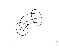
At time t the systems occupy the phase space volume dτ around the point with
coordinates (q1, . . . qi, . . . , q3N , p1, . . . pi, . . . , p3N ) (Fig. 1.5). The infinitesimal
3N
volume has the expression dτ = CN dpidqi, where CN is a constant that
i=1
only depends on N .
To compare this volume to the one at the instant t + dt, one has to evaluate
3N |
|
3N |
|
|
|
|
|
|
|
|
|
|
|
|
|
the products dpi(t)dqi(t) and |
dpi(t + dt)dqi(t + dt), that is, to calculate |
||||||
i=1 |
|
i=1 |
|
|
|
|
|
the Jacobian of the transformation |
|
|
|
|
(1.29) |
||
pi(t) → pi(t + dt) = pi(t) + dt · |
|
∂t |
|||||
|
|
|
|
|
|
∂pi(t) |
|
|
|
|
|
|
∂qi(t) |
|
|
|
|
|
|
|
|
|
|
qi(t) |
→ |
qi(t + dt) = qi(t) + dt |
· |
|
|
|
|
|
∂t |
|
|||||
|
|
|
|
|
|||
|
|
|
|
|
|
|
|
|
|
|
|
|
|
|
|
21
22 |
Appendix 1.1 |
pi 
t + dt
dτ
t
|
dτ |
O |
qi |
|
Fig. 1.5: The di erent systems, which were located in the volume dτ of the 6N -dimensional phase space at t, are in dτ at t + dt.
i.e., the determinant of the 6N × 6N matrix |
(t) |
|
|
||||
|
∂qj |
(t) |
|
∂qj |
|
||
|
∂qi(t + dt) |
|
∂pi(t + dt) |
|
|
||
|
∂qi(t + dt) |
|
∂pi(t + dt) |
|
(1.30) |
||
|
|
|
|
|
|
|
|
∂p |
(t) |
|
∂p |
(t) |
|
||
|
j |
|
|
j |
|
|
|
|
|
|
|
|
|
|
|
The Hamilton equations are used, which relate the conjugated variables qi and pi through the N -particle hamiltonian and are the generalization of Eq. (1.4) :
|
|
∂q |
|
|
∂H |
|||
|
i |
|
= |
|
|
|
|
|
|
∂t |
|
∂pi |
|||||
|
|
∂pi |
|
|
|
∂H |
||
|
|
|
|
|
|
|
|
|
|
|
|
|
= |
|
|
|
|
|
∂t |
− ∂qi |
||||||
|
|
|
||||||
|
|
|
|
|
|
|
|
|
One deduces |
|
|
|
|
|
|
|
|
|
qi(t + dt) = qi(t) + dt · |
∂H |
|||||
|
|
|
|
||||
|
∂pi |
||||||
|
|
|
|
|
|
∂H |
|
|
|
|
|
|
|
|
|
|
pi(t + dt) = pi(t) |
− |
dt |
· |
|
|
|
|
|
∂qi |
|||||
|
|
|
|
||||
|
|
|
|
|
|
|
|
and in particular |
|
|
|
|
|
|
|
|
∂qi(t + dt) |
= δij + dt · |
∂2H |
|||||
∂qj (t) |
|
∂qj ∂pi |
||||||
|
∂pi(t + dt) |
|
|
|
|
∂2H |
||
|
|
|
|
|
|
|
|
|
|
|
|
= δij |
|
dt |
|
|
|
∂pj (t) |
− |
· ∂pj ∂qi |
||||||
|
|
|
||||||
|
|
|
|
|
|
|
|
|
|
|
|
|
|
|
|
|
|
(1.31)
(1.32)
(1.33)
Appendix 1.1 |
23 |
The obtained determinant is developed to first order in dt :
Det(1 + dt · |
ˆ |
|
|
ˆ |
2 |
) |
|
M ) = 1 + dt |
· Tr M + O(dt |
||||||
with |
|
|
|
|
|
|
|
ˆ |
3N ∂2H |
|
3N ∂2H |
|
|
||
Tr M = − |
|
|
+ |
|
|
= 0 |
(1.34) |
|
∂pi∂qi |
|
∂pi∂qi |
||||
|
i=1 |
|
i=1 |
|
|
||
Consequently, the volume around a point of the 6N -dimensional phase space is conserved during the time evolution of this point; the number of systems in this volume, i.e., D(. . . qi, . . . , . . . pi, . . . , t)dτ , is also conserved.
B. Number of systems versus time in a fixed |
volume dτ |
|
of the phase space |
|
|
|
3N |
|
i |
|
|
In the volume dτ = CN |
dqi · dpi, at time t, the number of systems present |
|
is equal to |
=1 |
|
|
|
|
D(q1, . . . qi, . . . q3N , p1, . . . pi, . . . p3N )dτ |
(1.35) |
|
Each system evolves over time, so that it may leave the considered volume while other systems may enter it.
p1
q˙1(t)dt
dq1
dp 1
1
 (q˙1(t) + ∂q˙1(t) dq1) dt ∂q1
O |
q1 |
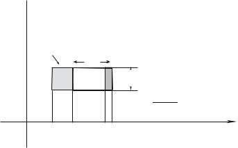
Fig. 1.6: In the volume dq1 · dp1 (thick line), between the times t and t + dt, the systems which enter were in the light grey rectangle at t ; those which leave the volume were in the dark grey hatched rectangle. It is assumed that q˙1(t) is directed toward the right.
Takea “box”, like the one in Fig. 1.6 which represents the situation for the only coordinates q1, p1. If only this couple of conjugated variables is considered, the

24 |
Appendix 1.1 |
problem involves a single coordinate q1 in real space (so that the velocity q˙1 is necessarily normal to the “faces” at constant q1) and we determine the variation of the number of systems on the segment for the q1 coordinate
[q1, q1 + dq1].
Considering this space coordinate, between the times t and t + dt, one calculates the di erence between the number of systems which enter the volume through the faces normal to dq1 and the number which leave through the same faces : the ones which enter were at time t at a distance of this face smaller or equal to q˙1(t)dt (light grey area on the Fig.), their density is D(q1 −dq1, . . . qi, . . . q3N , p1, . . . pi, . . . p3N ). Those which leave were inside the
area). |
Åq˙1 |
|
∂q1 |
1 |
ã |
|
volume, at a distance |
|
(t) + |
∂q˙1(t) |
dq |
|
dt from the face (dark grey hatched |
|
|
|
||||
The resulting change, between t and t + dt and for this set of faces, of the number of particles inside the considered volume, is equal to
− |
∂(q˙1(t)D) |
dq1dt |
(1.36) |
∂q1 |
For the couple of “faces” at constant p1, an analogous evaluation is performed, also contributing to the variation of the number of particles in the considered “box.” Now at 3N dimensions, for all the “faces,” the net increase of the number of particles in dτ during the time interval dt is
3N |
∂(Dq˙i(t)) |
dqidt − |
3N ∂(Dp˙i(t)) |
|
(1.37) |
|
− |
|
|
|
dpidt |
||
∂qi |
|
∂pi |
||||
i=1 |
|
|
i=1 |
|
|
|
This is related to a change in the particle density in the considered volume through to ∂D∂t dtdτ . Thus the net rate of change is given by
∂D |
3N |
∂D |
∂D |
|
3N |
∂q˙i |
|
∂p˙i |
|
|
||
= −i=1 Å |
ã |
− i=1 D Å |
|
ã |
|
|||||||
|
|
q˙i + |
|
p˙i |
|
+ |
|
(1.38) |
||||
∂t |
∂qi |
∂pi |
∂qi |
∂pi |
||||||||
From the Hamilton equations, the factor of D is zero and the above equation is equivalent to
dt = |
∂t |
3N |
Å ∂qi q˙i + |
∂pi p˙iã |
= 0 |
(1.39) |
|
+ i=1 |
|||||||
dD |
∂D |
|
|
∂D |
∂D |
|
|
where dD(q1, . . . , qi, . . . q3N , p1, . . . , pi, . . . p3N ) is the time derivative of the dt
probability density when one moves with the representative point of the system in the 6N -dimensional phase space. This result is equivalent to the one of §A.