

Statistical physics (2005)
.pdf142 |
Chapter 6. General Properties of the Quantum Statistics |
e ects, of little importance for a large system. Then at a given x the properties are the same, and the wave function takes the same value, whether the particle arrives at this point directly or after having traveled one turn around before reaching x :
ψ(x + Lx) = ψ(x) |
(6.47) |
Lx
O
x
Fig. 6.3 : The segment [0, Lx] is closed on itself.
This condition is expressed on the progressive-wave type wave function (6.39) through
exp ikx(x + Lx) = exp ikxx |
(6.48) |
|||
for any x, so that the condition to be fulfilled is |
|
|||
kxLx = nx |
2π |
(6.49) |
||
that is, kx = n |
|
2π |
(6.50) |
|
|
|
|
||
x Lx |
|
|||
where nx is integer. The same argument is repeated on the y and z coordinates.
The wave vector k is again quantized, with basis vectors twice larger than for the condition i) above for stationary waves, the allowed values now being
k = |
Ånx |
Lx ny |
Ly |
nz |
Lz ã |
|
|
2π |
2π |
|
2π |
The integers nx, ny, nz are now positive, negative or null (Fig. the time-dependent wave function is written, to a phase,
1 |
|
|
|
2k2 |
|
Ψ(r, t) = √ |
|
|
exp i(k.r |
− ωt), with ω = ε = |
2m |
|
|||||
Ω |
|
|
|
||
(6.51)
6.4). Indeed
(6.52)
Changing the sign of k, thus of the integers ni, produces a new wave which propagates in the opposite direction and is thus physically di erent. If one of these integers is zero, this means that the wave is constant along this axis.
Free Particle in a Box; Density of States |
143 |
|
|
kz |
|
|
|
2π |
|
|
|
Ly |
|
π |
|
2π |
|
2 |
x |
|
|
L |
Lz |
||
|
|||
|
|
ky |
|
kx |
|
|
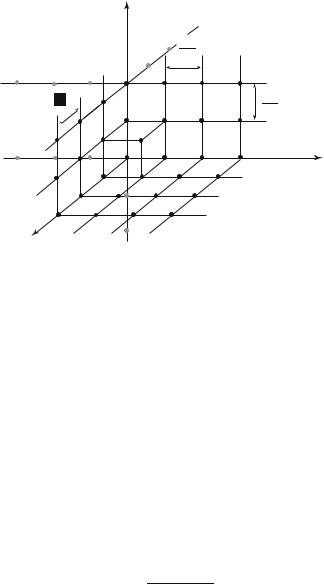
Fig.
6.4: Quantization of the k-space for the periodic (B-VK) boundary conditions. Note that each dimension of the elementary box is twice that corresponding to the stationary boundary conditions (Fig. 6.2), and that now the entire space should be considered.
6.4.2Density of States
Under these quantization conditions what is the order of magnitude of the obtained energies, and of the spacing of the allowed levels. As an example consider the framework of the periodic boundary conditions. The quantized allowed energies are given by
|
2 |
ñnx2 |
|
2π |
|
2 |
|
|
2π |
2 |
|
|
2π |
|
2 |
ô |
|
ε = |
|
Å |
|
ã |
|
+ ny2 |
Å |
|
ã |
+ nz2 |
Å |
|
ã |
|
(6.53) |
||
2m |
Lx |
|
Ly |
Lz |
|
For Lx for the order of 1 mm, a single coordinate and a mass equal to that of the proton,
2 |
|
2π |
ã |
2 |
= 13.6 eV. |
(2π)2 |
. |
|
0.5 × 10⁻¹⁰ |
ã |
2 |
8 |
|
10−16 |
eV (6.54) |
2m |
Å Lx |
|
1840 |
Å |
10−3 |
= |
× |
||||||||
|
|
|
|
|
|
||||||||||
For a mass equal to that of the electron, the obtained value, 1840 times larger, is still extremely small at the electron-volt scale!
The spacing between the considered energy levels is thus very small as compared to any realistic experimental accuracy, as soon as Lx is macroscopic, that is, large with respect to atomic distances (the Bohr orbit of the hydrogen atom is associated with energies in the electron-volt range, see the above es-

144 |
Chapter 6. General Properties of the Quantum Statistics |
timation). If the stationary boundary conditions had been chosen, the energy splitting would have been four times smaller.
The practical question which is raised is : “What is the number of available
3
quantum states in a wave vector interval d k around k fixed, or in an energy interval dε around a given ε ?” It is to answer this question that we are going to now define densities of states, which summarize the Quantum Mechanics properties of the system. It is only in a second step (§6.5) that Statistical Physics will come into play through the occupation factors of these accessible states.
a)Wave Vector and Momentum Densities of States (B-VK Conditions) :
One is estimating the number of quantum states dn of a free particle, confined
|
|
|
|
3 |
3 |
within a volume Ω, of wave vector between k and k + d |
k, the volume d k |
||||
being assumed to be large as compared to |
(2π)3 |
. The wave vector density of |
|||
|
Ω |
||||
|
|
|
|
|
|
states D (k) is defined by |
|
|
|
|
|
k |
|
|
|
|
|
|
|
3 |
|
|
(6.55) |
dn = D (k)d |
k |
|
|
||
k |
|
|
|
|
|
We know that the allowed states are uniformly spread in the k-space and that, in the framework of the B-VK periodic boundary conditions, for each
elementary volume (2π)3
Ω
parallelepiped has eight summits, shared between eight parallelepipeds. The searched number dn is thus equal to
3 |
|
|
Ω |
|
|
||
dn = |
d k |
|
3 |
|
|||
|
= |
|
|
(6.56) |
|||
(2π)3/Ω |
(2π)3 |
d k , |
|||||
which determines |
|
|
|
|
|
||
|
|
|
Ω |
|
|
|
|
|
D (k) = |
(2π)3 |
|
(6.57) |
|||
|
k |
|
|
||||
The above estimation has been done from the Schroedinger equation solutions related to the space variable r (orbital solutions). If the particle carries a spin s, to a given solution correspond 2s + 1 states with di erent spins, degenerate in the absence of applied magnetic field, which multiplies the above value of the density of states [Eq. (6.57)] by (2s + 1). Thus for an electron, of spin 1/2, there are two distinct spin values for a given orbital state. For a free particle, its wave vector and momentum are related by
|
3 |
p = |
3 |
3 |
(6.58) |
p = k d |
|
d |
k |

Free Particle in a Box; Density of States |
145 |
The number dn of states for a free particle of momentum vector between p and p + d3p, confined within the volume Ω, is written, from eq. (6.56),
dn = |
Ω d3p |
|
Ω |
|
|||
|
|
|
= |
|
d3p = Dp(p)d3p |
(6.59) |
|
(2π)3 |
3 |
h3 |
|||||
Here the (three-dimensional) momentum density of states has been defined through
Dp(p) = |
Ω |
(6.60) |
|
h3 |
|||
|
|
Note that the distance occupied by a quantum state, on the momentum axis of the phase space corresponding to the one-dimension motion of a single
h
particle, is Lx . This is consistent with the fact that a cell of this phase space
has the area h and that here ∆x = Lx, since, the wave function being of plane-wave type, it is delocalized on the whole accessible distance.
b) Three-Dimensional Energy Density of States (B-VK Conditions) :
The energy of a free particle only contains the kinetic term inside the allowed volume, it only depends of its momentum or wave vector modulus :
ε = |
2k2 |
|
p2 |
|||||
|
|
|
= |
|
|
|
(6.61) |
|
|
|
|
|
|||||
|
2m |
|
2m |
|||||
|
|
|
|
|
|
|
||
All the states corresponding to a given energy ε are, in the k-space, at the |
||||||||
surface of a sphere of radius k = |
|
|
2mε |
|
. If one does not account for the |
|||
|
|
2 |
||||||
…
particle spin, the number of allowed states between the energies ε and ε + dε
|
|
|
is the number of allowed values of k between the spheres of radii k and k + dk, |
||
dk being related to dε through dε = |
2 |
|
|
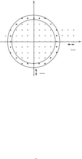
kdk. (For clarity in the sketch, Fig. |
|
|
||
|
m |
|
6.5 is drawn in the case of a two-dimensional problem.) |
||
The concerned volume is 4πk2dk, the number dn of the searched states, without considering the spin variable, is equal to
Ω |
4πk2dk = |
Ω |
|
4πk.kdk |
(6.62) |
|||||||
(2π)3 |
(2π)3 |
|||||||||||
|
|
|
|
|
|
|
|
|
||||
|
= |
2π2 |
… |
|
2 2 |
|
2 dε |
(6.63) |
||||
|
|
Ω |
|
|
|
mε m |
|
|||||
|
|
|
|
|
|
|
|
|
|
|
|
|
Thus a density of states in energy is obtained, defined by dn(ε) = D(ε) dε, with
|
|
|
(2 |
s + 1) |
|
2m |
|
3/2 |
||
D(ε) = CΩ√ε with C = |
Å |
ã |
(6.64) |
|||||||
|
|
|
||||||||
|
4π2 |
2 |
||||||||
146 |
Chapter 6. |
General Properties of the Quantum Statistics |
|
ky |
|
|
|
ε |
|
|
+ |
|
|
dε |
|
|
ε |
|
|
kx |
|
O |
2π |
|
|
Lx |
2π
Ly
Fig. 6.5: Number of states of energy between ε and ε + dε, (two-dimensional problem).
This expression of the energy density of states, which includes the spin degeneracy, is valid for any positive energy; the density of states vanishes for ε < 0, since then no state can exist, the energy being only of kinetic origin for the considered free particle.
c) Densities of States (Stationary-Waves Conditions)
We have seen that, in the case of stationary-wave conditions, all the physically distinct solutions are obtained when restricting the wave vectors choice to those with all three positive components. The volume corresponding to the states of energies between ε and ε + dε must thus be limited to the correspon-
ding trihedral of the k-space. This is the 1/8th of the space between the two spheres of radii k and k + dk, i.e., 18 4πk2dk, dk being still related to dε by
dε = |
2 |
(6.65) |
|
|
kdk |
||
|
|||
|
m |
|
|
However the wave vector density of states is eight times larger for the stationary-wave quantization condition than for the B-VK condition (the al-
lowed points of the k-space are twice closer in the x, y and z directions). Then one obtains a number of orbital states, without including the spin degeneracy, of
dn = |
Ω |
|
1 |
4πk2dk |
(6.66) |
|
π3 |
8 |
|||||
|
|
|
||||
Fermi-Dirac Distribution ; Bose-Einstein Distribution |
147 |
The density D(ε) thus has exactly the same value than in b) when the spin degeneracy (2s + 1) is introduced.
One sees that both types of quantization condition are equivalent for a macroscopic system. In most of the remaining parts of this course, the B-VK conditions will be used, as they are simpler because they consider the whole wave vector space. Obviously, in specific physical conditions, one may have to use the stationary-wave quantization conditions.
Notes :
In presence of a magnetic potential energy, which does not a ect the orbital
part of the wave function, the density of states D (k) is unchanged. On the
k
contrary, D(ε) is shifted (see §7.1.3).
As an exercise, we now calculate the energy density of states for free particles in the twoor one-dimension space. The relations between ε and k, between dε and dk are not modified [(6.61) and (6.65)].
– The two-dimension elementary area is 2πkdk, the k -density of states is given by L(2xπL)y2 without taking the spin in account and the energy density of states is a constant.
– In one dimension, the elementary length is 2dkx (kx and −kx correspond to the same energy, whence the factor 2), the kx-density of states is 2Lπ
1
without spin, and D(ε) varies like √ε . D(ε) diverges for ε tending to
zero but its integral, which gives the total number of accessible states from ε = 0 to ε = ε0, is finite.
6.5Fermi-Dirac Distribution ; Bose-Einstein Distribution
We have just seen that, for a macroscopic system, the accessible energy levels are extremely close and have defined a density of states, which is a discrete function of energy ε : in the large volume limit, it is as if D(ε) was a function of the continuous variable ε.
Let us now return to Statistical Physics in the framework of the large volumes limit. From the average number of occupation nk (see §6.3) of an energy level εk, one defines the energy function “ occupation factor” or “distribution,” of Fermi-Dirac or of Bose-Einstein according to the nature of the considered
148 Chapter 6. General Properties of the Quantum Statistics
particles : |
|
|
|
|
1 |
1 |
|
||
fF D(ε) = |
|
= |
|
(6.67) |
eβ(ε−µ) + 1 |
eβε−α + 1 |
|||
1 |
1 |
|
||
fBE (ε) = |
|
= |
|
(6.68) |
eβ(ε−µ) − 1 |
eβε−α − 1 |
|||
Recall that α and the chemical potential µ are related by α = βµ with
β = |
1 |
. |
|
||
|
kB T |
|
The consequences of the expression of their distribution will be studied in details in chapter 7 for free fermions and in chapter 9 for bosons.
6.6Average Values of Physical Parameters at T in the Large Volumes Limit
On the one hand, the energy density of states D(ε) summarizes the Quantum Mechanical properties of the system, i.e., it expresses the solutions of the Schroedinger equation for an individual particle. On the other hand, the distribution f (ε) expresses the statistical properties of the considered particles. To calculate the average value of a given physical parameter, one writes that in the energy interval between ε and ε + dε, the number of accessible states is D(ε)dε, and that at temperature T and for a parameter α or a chemical potential µ, these levels are occupied according to the distribution f (ε) (of Fermi-Dirac or Bose-Einstein). Thus
+∞ |
|
N = −∞ D(ε)f (ε) dε |
(6.69) |
+∞ |
|
U = −∞ εD(ε)f (ε) dε |
(6.70) |
The temperature and the chemical potential are included inside the distribution expression. In fact the first equation allows one to determine the chemical potential value.
To obtain the grand potential, one generalizes to a large system relations (6.31) and (6.32) that were established for discrete parameters :
+∞ |
|
A = +kB T −∞ D(ε) ln(1 − f (ε)) dε for fermions |
(6.71) |
A = −kB T +∞ D(ε) ln(1 + f (ε)) dε for bosons |
(6.72) |
−∞

Common Limit of the Quantum Statistics |
149 |
6.7Common Limit of the Quantum Statistics
6.7.1Chemical Potential of the Ideal Gas
In the case of free particles (fermions or bosons) of spin s, confined in a volume Ω, one expresses the number of particles (6.69) using the expression (6.64) of the density of states D(ε) :
|
(2s + |
1)Ω(2m)3/2 |
+∞ |
√ |
|
|
|
|
εdε |
|
|||||
N = |
|
0 |
|
(6.73) |
|||
|
4π2 3 |
eβε−α 1 |
|||||
where, in the denominator, the sign − is for bosons and the sign + for fermions. If the temperature is finite, the dimensionless variable of the integral is βε = x, so that this relation can be written :
N |
|
2mkB T |
|
3/2 (2s + 1) |
|
+∞ √ |
|
|
|
|||
= Å |
ã |
0 |
xdx |
(6.74) |
||||||||
Ω |
2 |
|
4π2 |
|
|
ex−α 1 |
||||||
The physical parameters are then put into the left member, which depends of the system density and temperature as
N 4π2 1 1 |
|
h2 |
|
3/2 |
|
N |
|
√ |
|
1 |
|
N |
λth3 |
|||||||
|
|
= |
π |
(λth)3 = constant |
||||||||||||||||
|
|
|
|
|
|
|
|
|
|
|
|
|
|
|
|
|
|
|||
|
|
|
|
|
|
|
Å mkB T |
ã |
|
|
|
|
|
|
|
|
||||
Ω (2π)3 2s + 1 23/2 |
|
|
Ω |
2 |
|
2s + 1 |
|
Ω(6.75) |
||||||||||||
The thermal de Broglie wavelength λth appears, as defined in §4.3. The quantity (6.75) must be equal to the right member integral, which is a function of α such that
∞ |
√ |
|
|
|
xdx |
|
|||
u (α) = 0 |
|
(6.76) |
||
ex−α 1 |
||||
√
In fact (6.75) expresses, to the factor π/2(2s+1), the cube of the ratio of the thermal de Broglie wavelength λth to the average distance between particles d = (Ω/N )1/3. It is this comparison which, in §4.3, had allowed us to define the limit of the classical ideal gas model. Since (6.75) and (6.76) are equal, one obtains :
|
1 |
|
√ |
|
|
|
N |
|
|
u (α) = |
π |
(λth)3 |
(6.77) |
||||||
|
|
|
|
|
|
|
|||
2s + 1 |
|
2 |
|
Ω |
|||||
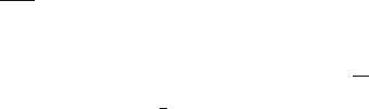
The integral u (α) can be numerically calculated versus α, it is a monotonous increasing function of α for either Fermi-Dirac (F D) or Bose-Einstein (BE) Quantum Statistics (Fig. 6.6). We already know the sign or the value of u(α) for some specific physical situations :
It was noted in §6.2.2 that the expression of f (ε) for Bose-Einstein statistics implies that α < βε1, i.e., α < 0 for free bosons, since then ε1 is zero. We
150 Chapter 6. General Properties of the Quantum Statistics
u±(α) |
uF D |
|
u+(α) = uF D u−(α) = uBE
uBE
constant NΩ λ3th
classical limit
αBE α |
O |
α |
F D |
|
Fig. 6.6: Sketch of the function u±(α) and determination of α from the physical data of the considered system.
will see in chapter 9 of this book that, in some situations, α vanishes, thus producing the Bose-Einstein condensation, which is a phase transition.
In the case of free fermions at low temperature, it will be seen in the next chapter that µ is larger than ε1, which is equal to zero, i.e., α > 0.
When α tends to minus infinity, the denominator term takes the same expression for both fermions and bosons. The integration is exactly performed :
u (α) eα 0+∞ √ |
|
|
√ |
|
1 |
|
|
π |
(6.78) |
||||||
xe−xdx = eα |
|||||||
2 |
|||||||
Considering the expression of the right member of 6.76, this limit does occur if the particle density n = N/Ω tends to zero or the temperature tends to infinity.
In the framework of this classical limit, one deduces
eα = |
N |
|
λth3 |
|
(6.79) |
|
Ω (2s + 1) |
||||||
|
|
|||||
which allows one to express the chemical potential µ, since α = µ/kB T . One
Common Limit of the Quantum Statistics |
|
|
|
|
151 |
||
finds, if the spin degeneracy is neglected, i.e., if one takes 2s + 1 = 1, |
|
||||||
µ = −kB T ln ñ |
Ω |
2πmk |
3/2 |
ô |
|
||
|
Å |
B T |
ã |
|
(6.80) |
||
N |
h2 |
|
|||||
the very expression obtained in §4.4.3 for the ideal gas.
6.7.2Grand Canonical Partition Function of the Ideal Gas
Let us look for the expression of A in the limit where α tends to minus infinity. For both fermions and bosons, one gets the same limit, by developing the Naperian logarithm to first order : it is equal to
A = −kB T |
eα−βεk |
(6.81) |
|
k |
|
= −kB T eα e−βεk |
(6.82) |
|
|
k |
|
One recognizes the one-particle partition function |
|
|
z1 = |
e−βεk |
(6.83) |
k |
|
|
(its value for the ideal gas was calculated in §4.4.1), whence |
|
|
A = −kB T eαz1 |
(6.84) |
|
By definition |
|
|
A = −kB T ln ZG, |
(6.85) |
|
thus in the common limit of both Quantum Statistics, i.e., in the classical limit conditions, ZG is equal to
ZG = exp(eαz1) = eαN |
zN |
|
||
1 |
|
(6.86) |
||
N ! |
||||
|
|
|||
N
Now the general definition of the grand canonical partition function ZG, using the N -particle canonical partition function ZcN , is
ZG = eαN ZcN |
(6.87) |
N |
|
This shows that in the case of identical particles, for sake of consistency, the N -particles canonical partition function must contain the factor 1/N !, the