Statistical physics (2005)

4.2Kinetic Approach

This section, which has no relation with Quantum Mechanics or Statistical Physics in equilibrium, will allow us to obtain insight into the simplest physical parameters describing the motion of molecules in a gas, and to introduce some orders of magnitude. If necessary, we will refer to the Thermodynamics courses on the ideal gas.

4.2.1Scattering Cross Section, Mean Free Path

Consider a can filled with a gas, in the standard conditions of temperature and pressure (T = 273 K, P = 1 atmosphere). Each molecule has a radius r, defined by the average extension of the valence orbitals, i.e., a fraction of a nanometer. If in its motion a molecule comes too close to another one, there will be a collision. One defines the scattering cross section which is the circle of radius r around a molecule, inside which no other molecule can penetrate.

r

d

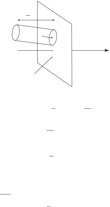
Fig. 4.1: Definitions of the scattering cross section and of the mean free path.

The mean distance between two collisions l, or mean free path, is deduced from the mean volume per particle Ω/N and the scattering cross section by

where d is the average distance between particles (Fig. 4.1). From l, one deduces the mean time τ between two collisions, or collision time, by writing

For nitrogen molecules with r = 0.42 nm, at 273 K and under a pressure of one atmosphere one finds l ≈ 70 nm, ν ≈ 300 m.sec−1, τ ≈ 2 × 10−10 sec. The length l is to be compared with the average distance between particles d = 3.3 nm. These values show that in the gas collisions are very frequent at the time scale of a measure, which ensures that equilibrium is rapidly reached after a perturbation of the gas; at the molecular scale distances covered between collisions are very large (of the order of a hundred times the size of a molecule), thus the motion of each molecule mostly occurs as if it was alone, that is, free.

4.2.2Kinetic Calculation of the Pressure

Let us now recall the calculation, from kinetic arguments, of the pressure of a gas, i.e., of the force exerted on a wall of unit surface by the molecules. The aim is to evaluate the total momentum transferred to this wall by the molecules impinging on it during the time interval ∆t : indeed in this chapter Classical Mechanics does apply, so that the total force on the wall is given by the Fundamental Equation of Dynamics :

i

Here the momentum brought by particle i is ∆pi. The resulting force is normal since the wall is at rest, it is related to the pressure P and to the considered wall surface S through

One will now evaluate the total momentum transferred to the surface, which is the di erence between the total momentum of the particles which reach the wall and that of the particles which leave it (Fig. 4.2).

The probability density in equilibrium f (r, pi, t) is assumed to be stationary, homogeneous, and isotropic in space (hypotheses stated by James Clerk Maxwell in 1859). It thus reduces to an even function f (p) versus the three components of the momentum and satisfies to

Consider the particles, of momentum equal to p to d3p, incident on the surface S during the time interval ∆t. They are inside an oblique cylinder along the

It is well known that the correct treatment of the particles motion must be done in Quantum Mechanics, so that the motion of a particle should not be described in terms of a trajectory but rather of a probability of presence deduced from a wave function. Moreover, the specific question raised by the Quantum Statistics, as will be seen in Chapter 5, is that of the indistinguishability of the particles.

But you also learnt that Classical Mechanics can however be used when the size of the considered system, here the average distance between two particles, is much larger than the characteristic dimension of the wave function, here its wavelength (in the opposite situation, the description in Quantum Mechanics is mandatory).

Let us first evaluate the characteristic dimension, at a given temperature T , of the wavelength of the molecules’ wave function. The momenta distribution is a function of T : it was just recalled that the mean kinetic energy per particle

of an ideal gas is equal to 32 kB T in thermal equilibrium at temperature T , which gives

to the root-mean-square value (4.15) of the momentum, one associates the wavelength λ of a free particle wave function, where h is the Planck constant. In order to simplify the forthcoming expressions of §4.4, the thermal de Broglie wavelength is defined here by

To know which of the Classical or Quantum Statistics applies, one thus compares λth to the averagedistance d between particles, of the order of (Ω/N )1/3.

Ω

If λth d, λ3th N , the classical statistics is applicable. Then

This is a high temperature or low density regime.

On the other hand, for λth ≥ d, the treatment of the present chapter is no longer valid and a quantum analysis is necessary (see Chapter 5 and following ones).

Take the example of a nitrogen gas in standard conditions of temperature and pressure : Ω = 22.4 liters for N = 6.02 × 1023 molecules and T = 273 K. The quantity to be compared to h = 6.63 × 10−34 J.sec is equal here to 1 × 10−31. Indeed the regime is classical. On the other hand, when at constant pressure the temperature is lowered to a few kelvins, the thermal L. de Broglie wavelength and the average distance between particles become comparable for gases of low atomic mass like helium (under the condition that they are not solid under these conditions!). In fact the right member of (4.19) is also written (kB T /P )1/3(2πmkB T )1/2 and thus varies like m1/2T 5/6. Classical Statistics is then no longer valid (see chapter 9).

In the next section we will study the ideal gas by the classical “MaxwellBoltzmann” statistics and thus assume that the condition λth d is fulfilled. Consequently, a classical description of the motion and of the phase space can be used (see §(1.1)) : until the next chapter we forget Quantum Mechanics...

4.4Classical Statistics Treatment of the Ideal Gas in the Canonical Ensemble

As explained in chapter 2, the statistical treatment of a macroscopic system will give the same physical results, whether performed in the microcanonical, canonical or grand canonical ensemble. In the ideal gas case, the microcanonical ensemble leads to somewhat more complicated calculations. The treatment could be done in the grand canonical ensemble; here we will choose the canonical ensemble. We follow the general method (see chapter 3) consisting in first calculating the canonical partition function Zc (§4.4.1), then deducing the average energy (§4.4.2) and the free energy F (§4.4.3) the partial derivatives of which provide the thermodynamical parameters pressure, entropy and chemical potential.

4.4.1Calculation of the Canonical Partition Function

We are concerned here by N monoatomic molecules, confined into a volume Ω, with energies reduced to their translational kinetic energies within this volume. Consequently, the probability of occurrence of the state in which the molecule i is within the volume d3ri around ri, with the momentum pi to

86 Chapter 4. The Ideal Gas

To express the confinement, the potential energy is taken as zero inside the volume Ω, infinite outside it. The canonical partition function for N particles, which normalizes the probabilities to unity, is calculated using the measure of the 6N -dimensional phase space introduced in §1.2.2 and expressed in the above formula. (Remember that CN is a constant which only depends on the number of particles.)

As already seen in §2.4.5 of chapter 2, since the total energy consists in a sum of similar one-particle terms, the partition function is a product of terms :

(Do not forget the CN factor of the phase space measure!)

If the potential only expresses that the molecule remains within the volume Ω, the integral in r1 is equal to Ω (the exponential is equal to one in the allowed volume, zero outside it).

Note : If the potential is position-dependent, as in the case of a gas in equilibrium in the gravity field, the probability of presence and the density both vary in exp(−βV (r)) and the integral in r1 is di erent from Ω (it is proportional to the characteristic extension of the potential energy).

From now we assume that the gas is confined, with a uniform probability of presence within the allowed volume.

The integral in momentum is reduced into the product of three Gaussian integrals, each one concerning a single coordinate :

88 Chapter 4. The Ideal Gas

For each of these terms, an integration by parts allows one to transform the

In fact this calculation is valid in the Maxwell-Boltzmann Classical Statistics for the average value of any energy term expressed as a quadratic degree of

freedom, for example an elastic potential energy of the type 12 kix2i , for which

ki > 0. Indeed one will always perform an integration by parts of a seconddegree term in energy in the numerator to express the corresponding factor of the denominator partition function, which will provide the factor kB T /2. But this property is not valid for a polynomial of degree di erent than two, for example for an anharmonic term in x3i .

This result constitutes the “theorem of energy equipartition”, established by James C. Maxwell as early as 1860 :

For a system in canonical equilibrium at temperature T , the average value of the energy per particle and per quadratic degree of

freedom is equal to 12 kB T .

We have already used this property several times, in particular in §4.3 to find the root-mean-square momentum of the ideal gas at temperature T . It is also useful to determine the thermal fluctuations of an oscillation, providing

a potential energy in 12 kx2 for a spring, in 12 Cϑ2 for a torsion pendulum,

and more generally to calculate the average value at temperature T of a hamiltonian of the form

ij

where ai is independent of xi, bj does not depend of pj , and all the coe - cients ai and bj are positive (which allows to use this property for an energy development around a stable equilibrium state).

A case of application of the energy equipartition theorem is the specific heat at constant volume associated to U . We recall its expression

Å ∂U ã

Cv = (4.34)

∂T Ω,N