

Statistical physics (2005)
.pdf152 |
Chapter 6. General Properties of the Quantum Statistics |
“memory” of the Quantum Statistics, to take into account the indistinguishability of the particles :
ZcN = |
1 |
|
zN |
(6.88) |
|
N ! |
|||||
|
1 |
|
|||
This factor ensures the extensivity of the thermodynamical functions, like S, and allows to solve the Gibbs paradox (there is no extra entropy when two volumes of gases of the same density and the same nature are allowed to mix into the same container.) (see §4.4.3).
Notes :
The above reasoning allows one to grasp how, in the special case of free particles, one goes from a quantum regime to a classical one.
We did not specify to which situation corresponds the room temperature, the most frequent experimental condition. We will see that for metals, for example, it corresponds to a very low temperature regime, of quantum nature (see chapter 7).

Summary of Chapter 6
To account for the occupation conditions of the energy states as stated by the Pauli principle, it is simpler to work in the grand canonical ensemble, in which the number of particles is only given in average : then, at the end of the calculation, the value of the chemical potential is adjusted so that this average number coincides with the real number of particles in the system. As soon as the system is macroscopic, the fluctuations around the average particle number predicted in the grand canonical ensemble are much smaller than the resolution of any measure.
The grand partition function gets factorized by energy level and takes a different expression for fermions and for bosons.
Remember the distribution, which provides the average number of particles, of chemical potential equal to µ, on the energy level ε at temperature T = 1/kBβ :
for fermions |
1 |
|
|
fF D(ε) = |
|
(6.89) |
|
|
|
||
exp β(ε − µ) + 1 |
|||
for bosons |
1 |
|
|
fBE (ε) = |
|
(6.90) |
|
|
|
||
exp β(ε − µ) − 1 |
|||
For a free particle in a box, we calculated the location of the allowed energy levels. The periodic boundary conditions of Born-Von Kármán (or in an analogous way the stationary-waves conditions) evidence quantized levels, and for a box of macroscopic dimensions (“large volume limit”), the allowed levels are extremely close. One then defines an energy density of states such that the number of allowed states between ε and ε + dε is equal to
dn = D(ε)dε |
(6.91) |
For a free particle in the three-dimensional space D(ε) √ε.
153
154 |
Summary of Chapter 6 |
In the large volume limit the average values at temperature T of physical parameters are expressed as integrals, which account for the existence of allowed levels through the energy density of states and for their occupation by the particles at this temperature through the distribution term :
+∞ |
|
N = −∞ D(ε)f (ε) dε |
(6.92) |
+∞ |
|
U = −∞ εD(ε)f (ε) dε |
(6.93) |
We showed how for free particles the Classical Statistics of the ideal gas is the common limit of the Fermi-Dirac and Bose-Einstein statistics when the temperature is very high and/or the density very low. The factor 1/N ! in the canonical partition function of the ideal gas is then the “memory” of the Quantum Statistics properties.

Chapter 7
Free Fermions Properties
We now come to the detailed study of the properties of the Fermi-Dirac quantum statistics. First at zero temperature we will study the behavior of free fermions, which shows the consequences of the Pauli principle. Then we will be concerned by electrons, considered as free, and will analyze two of their properties which are temperature-dependent, i.e., their specific heat and the “ thermionic” emission. In the next chapter we will understand why this free electron model indeed properly describes the properties of the conduction electrons in metals.
In fact, in the present chapter we follow the historical order : the properties of electrons in metals, described by this model, were published by Arnold Sommerfeld (electronic specific heat, Spring 1927) and Wolfang Pauli (electrons paramagnetism, December 1926), shortly after the statement of the Pauli principle at the beginning of 1925.
7.1Properties of Fermions at Zero Temperature
7.1.1Fermi Distribution, Fermi Energy
The Fermi-Dirac distribution, presented in §6.5, gives the average value of the occupation number of the one-particle state of energy ε, and is a function of the chemical potential µ. Its expression is
f (ε) = |
1 |
= |
1 |
ï |
1 |
− |
tanh |
β(ε − µ) |
(7.1) |
|
eβ(ε−µ) + 1 |
2 |
2 |
||||||||
|
|
|
|
ò |
155
156 |
Chapter 7. Free Fermions Properties |
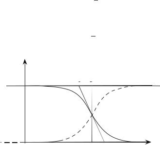
It is plotted in Fig. 7.1 and takes the value 12 for ε = µ for any value of β and
thus of the temperature. This particular point is a center of inversion of the curve, so that the probability of “nonoccupation” for µ−δε, i.e., 1 −f (µ−δε), has the same value as the occupation probability for µ + δε, i.e., f (µ + δε).
At the point ε = µ the tangent slope is −β4 : the lower the temperature, the larger this slope.
f |
|
|
|
|
1 − f |
2 kB T |
|
||
1 |
|
|
1 |
− f (ε) |
|
||||
f (ε)
0 |
|
|
|
µ |
ε |
||
Fig. 7.1 : Variation versus energy of f (ε) and 1 − f (ε).
In particular when T tends to zero, f (ε) tends to a “step function” (Heaviside function). One usually calls Fermi energy the limit of µ when T tends to zero ; it is noted εF , its existence and its value will be specified below. Then one obtains at T = 0 :
®
f (ε) = 1 |
if ε < εF |
(7.2) |
|
f (ε) = 0 |
if ε > εF |
||
|
At T = 0 K the filled states thus begin at the lowest energies, and end at εF , the last occupied state. The states above εF are empty. This is in agreement with the Pauli principle : indeed in the fundamental state the particles are in their state of minimum energy but two fermions from the same physical system cannot occupy the same quantum state, whence the requirement to climb up in energy until the particles all located.
In the framework of the large volume limit, to which this course is limited, the total number N of particles in the system satisfies
∞ |
|
N = D(ε)f (ε)dε |
(7.3) |
0
where D(ε) in the one-particle density of states in energy. This condition determines the µ value.
Properties of Fermions at Zero Temperature |
157 |
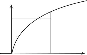
At zero temperature, the chemical potential, then called the “Fermi energy εF ,”, is thus deduced from the condition that
εF
N = |
D(ε)dε |
(7.4) |
0
The number N corresponds to the hatched area of Fig. 7.2.
|
|
) |
|
ε |
|
( |
|
|
D |
|
|
f (ε)
T = O K
0 |
εF |
ε |
Fig. 7.2: Density of states D(ε) of three-dimensional free particles and determination of the Fermi energy at zero temperature. The hatched area under the curve provides the number N of particles in the system.
For a three-dimensional system of free particles, with a spin s = 1/2, from (6.64)
D(ε) = |
|
Ω |
|
|
(2m)3/2√ |
|
|
|
for |
ε > 0 |
||||||
|
|
|
ε |
|||||||||||||
|
2π2 3 |
|||||||||||||||
|
|
|
|
|
|
|
|
|
|
|
|
|
(7.5) |
|||
D(ε) = 0 |
|
|
|
|
|
|
|
|
|
|
|
|
for |
ε ≤ 0 |
||
The integral (7.4) is then equal to |
|
|
|
|
|
|
|
|
|
|||||||
|
N = |
2 |
|
Ω |
|
(2m)3/2 |
3/2 |
(7.6) |
||||||||
|
|
|
|
|
εF |
|||||||||||
|
3 |
2π2 3 |
||||||||||||||
that is, |
|
|
|
|
|
|
|
|
|
|
|
|
|
|
|
|
|
|
|
|
|
|
2 |
Å3π2 |
|
N |
ã |
2/3 |
|
||||
|
|
εF = |
|
|
|
|
(7.7) |
|||||||||
|
|
|
|
|
|
|
|
|
||||||||
|
|
|
2m |
Ω |
|
|
||||||||||
This expression leads to several comments :
158 |
Chapter 7. Free Fermions Properties |
–N and Ω are extensive, thus εF is intensive;
–εF only depends on the density N/Ω ;
–the factor of 2/2m in (7.7) is equal to kF2 , where kF is the Fermi wave
vector : in the k-space the surface corresponding to the constant energy εF , called “Fermi surface,” contains all the filled states. In the case of
free particles, it is a sphere, the “Fermi sphere,” of radius kF . One can |
||||||||||||||
also define the momentum pF = |
|
kF |
√ |
|
|
|
|
|
|
|||||
|
|
|
|
|
|
|||||||||
|
|
= |
2mεF . Then expression (7.6) |
|||||||||||
can be obviously expressed versus kF or pF for spin-1/2 particles : |
||||||||||||||
N = |
2Ω |
|
4 |
πk3 |
= |
2Ω |
|
4π |
p3 |
(7.8) |
||||
|
|
|
|
|||||||||||
|
(2π)3 |
3 |
|
F |
|
h3 3 |
F |
|
||||||
|
|
|
|
|
|
|||||||||
The first factor is equal to D (k) (resp. Dp(p)), the one-particle density
k
of states in the wave vector- (resp. momentum-) space. Expression (7.8) is also directly obtained by writing :
kF
3 N = D (k)d k .
k
0
–εF corresponds, for metals, to energies of the order of a few eV. Indeed, let us assume now (see next chapter) that the only electrons to be considered are those of the last incomplete shell, which participate in the conduction. Take the example of copper, of atomic mass 63.5 g
and density3 |
9 g/cm3. There are thus 9N/63.5 = 0.14N copper atoms |
|||
per cm , N being the Avogadro number. Since one electron per copper3 |
||||
atom participates in conductivity, the number of such electrons per cm |
||||
is of 0.14N = 8.4 × 10²²/cm3 |
i.e., 8.4 × 1028/ m3. This corresponds to |
|||
a wave vector kF = 1.4 × 10¹⁰ |
m−1, and to a velocity at the Fermi level |
|||
vF = |
kF |
of 1.5 × 10⁶ m/sec. One deduces εF = 7 eV. |
||
m |
||||
Remember that the thermal energy at 300 K, kB T , is close to 25 meV, so that the Fermi energy εF corresponds to a temperature TF such that kB TF = εF , in the 104 or 105 K range according to the metal (for copper 80, 000 K)!
7.1.2Internal Energy and Pressure of a Fermi Gas at Zero Temperature
The internal energy at zero temperature is given by
εF
U = |
εD(ε)dε |
(7.9) |
0

Properties of Fermions at Zero Temperature |
159 |
For the three-dimensional density of states (7.5), U is equal to :
U = |
|
2 |
|
Ω |
|
|
(2m)3/2 |
εF5/2 |
(7.10) |
|
5 |
|
2π2 3 |
||||||||
|
|
|
|
|
|
|||||
i.e., by expressing N using (7.6), |
|
|
|
|
|
|
|
|||
|
|
|
|
U = |
3 |
N εF |
|
(7.11) |
||
|
|
|
|
|
|
|||||
|
|
|
|
5 |
|
|||||
Besides, |
|
|
|
|
|
|
|
|
|
|
|
P = − Å |
∂U |
|
|
||||||
|
|
ãN |
|
(7.12) |
||||||
|
∂Ω |
|
||||||||
From (7.10) and (7.7), U varies like N 5/3Ω−2/3, so that at constant particles number N
P = |
2 U |
(7.13) |
|||
|
|
|
|||
3 Ω |
|||||
|
|
||||
For copper, one obtains P = 3.8 × 10¹⁰ N/m2 = 3.7 × 10⁵ atmospheres. This very large pressure, exerted by the particles on the walls of the solid which contains them, exists even at zero temperature. Although the state equation (7.13) is identical in the cases of fermions and of the ideal gas, the two situations are very di erent : for a classical gas, when the temperature tends to zero, both the internal energy and the pressure vanish. For fermions, the Pauli principle dictates that levels of nonzero energies are filled. The fact that electrons in the same orbital state cannot be more than a pair, and of opposite spins, leads to their mutual repulsion and to a large average momentum, at the origin of this high pressure.
7.1.3Magnetic Properties. Pauli Paramagnetism
A gas of electrons, each of them carrying a spin magnetic moment equal to
the Bohr magneton µB , is submitted to an external magnetic field B. If N+
is the number of electrons with a moment projection along B equal to +µB , N− that of moment −µB , the gas total magnetic moment (or magnetization)
along B is
M = µB (N+ − N−) |
(7.14) |
The density of states D (k) is the same as for free electrons. Since the potential
k
energy of an electron depends on the direction of its magnetic moment, the total energy of an electron is
|
2 2 |
|
|
ε± = |
k |
µB B |
(7.15) |
2m |
160 |
Chapter 7. Free Fermions Properties |
The densities of states D+(ε) and D−(ε) now di er for the two magnetic moment orientations, whereas in the absence of magnetic field,
D+(ε) = D−(ε) = D(ε)/2 : here
®
D+(ε) |
= |
1 D(ε + µB B) |
(7.16) |
|
|
|
2 |
||
D−(ε) |
= 21 D(ε − µB B) |
|||
|
||||
Besides, the populations of electrons with the two orientations of magnetic moment are in equilibrium, thus they have the same chemical potential.
The solution of this problem is a standard exercise of Statistical Physics. Here we just give the result, in order to comment upon it : one obtains the magnetization
M = µB · µB B · D(εF ) |
(7.17) |
This expresses that the moments with the opposite orientations compensate, except for a small energy range of width µB B around the Fermi energy. The
|
|
|
|
|
|
|
|
|
|
|
|
|
|
|
|
|
|
1 |
|
|
|
corresponding (Pauli) susceptibility, defined by lim |
|
M |
, is equal to |
||||||||||||||||||
|
µ Ω |
|
|||||||||||||||||||
|
|
|
|
|
|
|
|
|
|
|
|
|
|||||||||
|
|
|
|
|
|
|
|
|
|
|
|
|
|
|
B→0 |
0 |
|
B |
|
||
χ = |
1 3 N µB2 |
= |
1 3 N µB2 |
kB T |
|
|
(7.18) |
||||||||||||||
|
|
|
|
|
|
|
|
|
|
|
|
|
|
· |
|
|
|
|
|||
µ0 |
2 |
Ω |
εF |
µ0 |
2 |
Ω |
kB T |
|
εF |
|
|
||||||||||
with µ0 = 4π × 10−7. It is reduced with respect to the classical result (Curie law) by a factor of the order of kB T /εF , which expresses that only a very small fraction of the electrons participate in the e ect (in other words, only a few electrons can reverse their magnetic moment to have it directed along the external field).
7.2Properties of Fermions at Non-Zero Temperature
7.2.1Temperature Ranges and Chemical Potential Variation
At nonvanishing temperature, one again obtains the chemical potential µ position from expression (7.3), which links µ to the total number of particles :
∞
N = D(ε)f (ε)dε
0
∞ |
1 |
|
|
|
= 0 |
D(ε) |
|
dε |
(7.3) |
eβ(ε−µ) + 1 |
||||
Properties of Fermions at Non-Zero Temperature |
161 |
|
) |
(ε |
|
D |
|
f (ε)
T TF
 f (ε)D(ε)
0 |
µ εF |
ε |
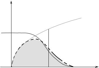
Fig. 7.3 : Determination of the chemical potential µ for T TF .
Relation (7.3) implies that µ varies with T . Fig. 7.3 qualitatively shows for kB T εF the properties which will be calculated in Appendix 7.1. Indeed the area under the curve representing the product D(ε)f (ε) gives the number of particles. At T = 0 K, one has to consider the area under D(ε) up to the energy εF ; at small T , a few states above µ are filled and an equivalent number below µ are empty. Since the function D(ε) is increasing, to maintain
an area equal to N, µ has to be smaller than εF , of an amount proportional to D (µ).
The exact relation allowing one to deduce µ(T ) for the two Quantum Statistics was given in (6.74) : recalling that α = βµ, and substituting (7.5) into (7.3) one obtains for fermions
∞ |
√ |
|
|
|
|
|
N |
|
|
|
2 |
3/2 |
|
||
xdx |
= 2π2 |
|
|
|
|
(7.19) |
|||||||||
0 |
exp(x − α) + 1 |
· |
|
Ω |
Å |
3/2 B |
ã |
||||||||
|
|
|
|
|
|
|
|
|
|
|
|
|
2mk T |
|
|
|
|
|
|
= |
2 |
Å |
|
εF |
|
ã |
|
(7.20) |
|||
|
|
|
|
3 |
kB T |
|
|
||||||||
In the integral we defined βε = x.
Thus α is related to the quantity εF /kB T = TF /T .
–When T vanishes, the integral (7.19) tends to infinity : the exponential in the denominator no longer plays any role since α tends to infinity (εF is finite and β tends to infinity). The right member also tends to