

Statistical physics (2005)
.pdfAppendix 7.1
but µ depends on T since
µ |
|
π2 |
|
N = 0 |
Kε1/2dε + |
|
(kB T )2(Kε1/2)µ + O(T 4) = |
6 |
|||
expresses the conservation of the particles number. One deduces from (7.50) :
εF
Kε1/2dε
0
µ(T ) = εF ñ1 − π2 Å kB T ã2ô + O(T 4) 12 εF
Replacing the expression of µ(T ) into U (T ), one gets :
|
5/2 π2 |
|
Å |
kB T |
|
|
2 |
|
|
|
π2 |
Å |
kB T |
|
2 |
|||
|
|
|
ã = N εF |
ã |
|
|||||||||||||
U (T ) − U (T = 0) KεF |
|
|
|
|
|
|
|
|
||||||||||
6 |
|
εF |
|
4 |
εF |
|
||||||||||||
One deduces Cv : |
|
|
|
|
|
|
|
|
|
|
|
|
|
|
|
|
|
|
Cv = |
dU |
= |
3 |
N kB |
· |
π2 |
Å |
kB T |
ã |
|
|
|
|
|||||
dT |
2 |
3 |
εF |
|
|
|
|
|||||||||||
173
(7.50)
(7.51)
(7.52)
(7.53)
Chapter 8
Elements of Bands Theory
and Crystal Conductivity
The previous chapter on free fermions allowed us to interpret some properties of metals. We considered that each electron was confined within the solid by potential barriers, but did not introduce any specific description of its interactions with the lattice ions or with the other electrons. This model is not very realistic, in particular it cannot explain why some solids are conducting the electrical current and others are not : at room temperature, the conductivity of copper is almost 108 siemens (Ω−1 · m−1) whereas that of quartz is of 10−15 S, and of teflon 10−16 S. This physical parameter varies on 24 orders of magnitude according to the material, which is absolutely exceptional in nature.
Thus we are going to reconsider the study of electrons in solids from the start and to first address the characteristics of a solid and of its physical description. As we now know, the first problem to solve is a quantum mechanical one, and we will rely on your previous courses. In particular we will be concerned by a periodic solid, that is, a crystal (§8.1). We will see that the electron eigenstates are regrouped into energy bands, separated by energy gaps (§8.2 and §8.3).
We will have to introduce here very simplifying hypotheses : in Solid State Physics courses, more general assumptions are used to describe electronic states of crystals.
Using Statistical Physics (§8.4) we will see how electrons are filling energy bands. We will understand why some materials are conductors, other ones insulators. We will go more into details on the statistics of semiconductors,
175
176 |
Chapter 8. Elements of Bands Theory and Crystal Conductivity |
of high importance in our everyday life, and will end by a brief description of the principles of a few devices based on semiconductors (§8.5).
8.1What is a Solid, a Crystal ?
A solid is a dense system with a specific shape of its own. This definition expresses mechanical properties; but one can also refer to the solid’s visual aspect, shiny in the case of metals, transparent in the case of glass, colored for painting pigments. These optical properties, as well as the electrical conduction and the magnetic properties, are due to the electrons. In a macroscopic solid with a volume in the cm3 range, the numbers of electrons and nuclei present are of the order of the Avogadro number N = 6.02 × 10²³.
The hamiltonian describing this solid contains for each particle, either electron or nucleus, its kinetic energy, and its potential energy arising from its Coulombic interaction with all the other charged particles. It is easily guessed that the exact solution will be impossible to get without approximations (and still very di cult to obtain using them!).
One first notices that nuclei are much heavier than electrons and, consequently, much less mobile : either the nuclei motion will be neglected by considering that their positions remain fixed, or the small oscillations of these nuclei around their equilibrium positions (solid vibrations) will be treated se-
ˆ
parately from the electron motions, so that the electron hamiltonian H will
ˆ
not include the nuclei kinetic energy. H will then be given by
N Z |
ˆ2 |
|
|
2 |
N Z N |
1 |
|
|
|
1 |
|
|
2 |
|
N Z |
1 |
|
|
||
ˆ |
pi |
|
Ze |
|
|
|
|
|
|
+ |
|
e |
|
|
|
|
|
|||
H = |
2m |
− |
4πε |
|
| |
− |
|
| |
2 |
|
4πε |
|
|
r |
r |
(8.1) |
||||
i=1 |
|
|
|
|
0 |
Rn |
|
|
|
|
|
0 i,j=1 | i − |
j | |
|
||||||
|
|
|
|
i=1 n=1 ri |
|
|
|
|
|
|
|
|
||||||||
where Z is the nuclear charge; the nth nucleus is located at Rn and the electron i at ri. The second term expresses the Coulombian interaction of all the electrons with all the nuclei, the third one the repulsion among electrons.
Besides, we will assume that the solid is a perfect crystal, that is, its atoms are
regularly located on the sites Rn of a three-dimensional periodic lattice. This will simplify the solution of the Quantum Mechanical problem, but many of our conclusions will also apply to disordered solids.
ˆ
The repulsion term between electrons in H depends of their probabilities of presence, in turn given by the solution of the hamiltonian : this is a di cult self-consistent problem. The Hartree method, which averages the electronic repulsion, and the Hartree-Fock method, which takes into account the wave function antisymmetrization as required by the Pauli principle, are used to
The Eigenstates for the Chosen Model |
177 |
ˆ |
N |
ˆ |
|
|
(8.2) |
||
H = |
|
hi |
|
|
i=1 |
|
|
with |
|
|
|
ˆ |
ˆ2 |
|
|
pi |
+ V(ri) |
|
|
hi = |
|
(8.3) |
|
2m |
The potential V(ri) has the lattice periodicity, it takes into account the attractions and repulsions on electron i and is globally attractive. The eigenvalues
ˆ
of H are the sums of the eigenenergies of the various electrons.
ˆ
Our task will consist in solving the one-electron hamiltonian hi. We will introduce an additional simplification by assuming that the lattice is onedimensional, i.e., V(ri) = V(xi). This will allow us to extract the essential characteristics, at the cost of simpler calculations.
In the “electron in the box” model that we have used up to now, V(xi) only expressed the potential barriers limiting the solid, and thus leveled out the potential of each atom. Here we will introduce the attractive potential on each lattice site. The energy levels will derive from atomic levels, rather than from the free electron states which were the solutions in the “box” case.
8.2The Eigenstates for the Chosen Model
8.2.1Recall : the Double Potential Well
First consider an electron on an isolated atom, located at the origin. Its ha-
ˆ
miltonian h is given by
ˆ |
pˆ2 |
|
|
h = |
2m |
+ V (x) |
(8.4) |
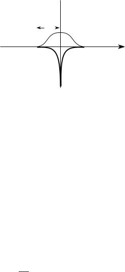
where V is the even Coulombian potential of the nucleus (Fig. 8.1).
178 |
Chapter 8. Elements of Bands Theory and Crystal Conductivity |
One of its eigenstate is such that :
ˆ |
ϕ(x) |
(8.5) |
hϕ(x) = ε0 |
ϕ(x) is an atomic orbital, of s-type for example, which decreases from the origin with a characteristic distance λ. We will assume that the other orbitals do not have to be considered in this problem, since they are very distant in energy from ε0.
 V
V
λ |
2 |
|
|
|ϕ| |
|
|
||
|
|
|
x
Fig. 8.1: Coulombian potential of an isolated ion and probability of presence of an electron on this ion.
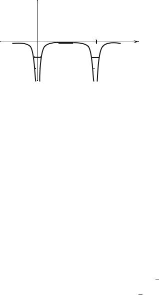
Let us add another nucleus, that we locate at x = d (Fig. 8.2). The hamiltonian, still for a single electron now sharing its presence between the two ions,
ˆ |
pˆ2 |
|
|
h = |
|
+ V (x) + V (x − d) |
(8.6) |
2m |
|||
In the case of two 1s-orbital initial states, this corresponds to the description of the H+2 ion (two protons, one electron).
One follows the standard method on the double potential well of the Quantum Mechanics courses and defines |ϕL and |ϕR , the atomic eigenstates respectively located on the left nucleus (at x = 0 ) and the right nucleus (at x = d) :
2m + V (x) |ϕL |
= ε0|ϕL |
|||
ñ |
pˆ2 |
ô |
|
(8.7) |
|
|
|
|
|
|
|
|
|
|
|
|
|
|
|
|
2 |
|
|
|
|
pˆ |
+ V (x − d) |
|ϕR = ε0|ϕR |
|
|
2m |
|||
ï |
|
|
ò |
|
The Eigenstates for the Chosen Model |
179 |
 V
V
0 |
d |
x
ε0 + A
ε0 − A
Fig. 8.2: Potential due to two ions of the same nature, distant of d and corresponding bound states.
Owing to the symmetry of the potential in (8.6) with respect to the point
ˆ
x = d/2, whatever d the eigenfunctions of h can be chosen either symmetrical or antisymmetrical with respect to this mid-point. However, if d is very large
ˆ
with respect to λ, the coupling between the two sites is very weak, h has two eigenvalues practically equal to ε0 and if at the initial time the electron is on one of the nuclei, for example the left one L, it will need a time overcoming the observation possibilities to move to the right one R. One can then consider that the atomic states (8.7) are the eigenstates of the problem (although strictly they are not).
On the other hand, you learnt in Quantum Mechanics that if d is not too large with respect to λ, the L and R wells are coupled by the tunnel e ect, which is expressed through the coupling matrix element
ˆ |
(8.8) |
−A = ϕR|H|ϕL , A > 0 |
which decreases versus d approximately like exp(−d/λ).
ˆ
The energy degeneracy is then lifted : the two new eigenvalues of h are equal
1
to ε0 −A, corresponding to the symmetrical wave function |ψS = √ (|ϕL + 2
1
|ϕR ), and ε0 + A, of antisymmetrical wave function |ψA = √ (|ϕL − |ϕR ) 2
(Fig. 8.2). These results are valid for a weak enough coupling (A |ε0|).
For a stronger coupling (d λ) one should account for the overlap of the two atomic functions, expressed by ϕL|ϕR di erent from zero. Anyway the eigenstates are delocalized between both wells. For H+2 they correspond to the bonding and antibonding states of the chemical bound.
180 |
Chapter 8. Elements of Bands Theory and Crystal Conductivity |
8.2.2Electron on an Infinite and Periodic Chain
In the independent electrons model, the hamiltonian describing a single electron in the crystal is given by
ˆ |
pˆ2 |
+∞ |
|
|
hcrystal = |
|
+ |
V (x − xn) |
(8.9) |
2m |
||||
|
|
|
n=−∞ |
|
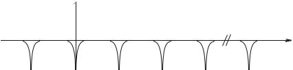
where xn = nd, is the location of the nth nucleus. The potentials sum is periodic and plays the role of V(ri) in formula (8.3) (Fig. 8.3).
 V
V
0 |
d |
2d |
nd |
x
Fig. 8.3 : Potential periodic of a crystal.
One is looking for the stationary solution, such that
ˆ |
(8.10) |
hcrystalψ(x) = εψ(x) |
If the nuclei are far enough apart, there is no coupling : although the eigenstates are delocalized, if at the initial time the electron is on a given nucleus, an infinite time would be required for this electron to move to the neighboring nucleus. The state of energy ε = ε0 is N times degenerate. On the other hand, in the presence of an even weak coupling, the eigenstates are delocalized. We are going to assume that the coupling is weak and will note :
hˆcrystal = hˆn + n =n V (x − n d) |
(8.11) |
|
|
to show the atomic hamiltonian on the specific site n.
To solve the eigenvalue problem, by analogy with the case of the double potential well, we will work in a basis of localized states, which are not the eigenstates of the considered infinite periodic chain. Now every site plays a similar role, the problem is invariant under the translations which change x into x + nd = x + xn. The general basis state is written |n , it corresponds to the wave function φn(x) located around xn and is deduced through the translation xn from the function centered at the origin, i.e., φn(x) = φ0(x − xn).
These states are built through orthogonalization from the atomic functions ϕ(x − xn) in order to constitute an orthonormal basis : n |n = δnn (this is
The Eigenstates for the Chosen Model |
181 |
the so-called “Hückel model”). The functions φn(x) depend on the coupling. When the atoms are very distant, φn(x) is very close to ϕ(x −xn), the atomic wave function. In a weak coupling situation, where the tunnel e ect only takes place between first neighbors, φn(x) is still not much di erent from the atomic function.
One looks for a stationary solution of the form |
|
|
|ψ = |
cn|n |
(8.12) |
|
n |
|
One needs to find the coe cients cn, expected to all have the same norm, since every site plays the same role :
+∞ |
+∞ |
|
hˆcrist n=−∞ cn|n |
= ε n=−∞ cn|n |
(8.13) |
One proceeds by analogy with the solution of the double-well potential problem : one assumes that the hamiltonian only couples the first neighboring sites. Then the coupling term is given by
ˆ |
ˆ |
(8.14) |
n|hcrist|n + 1 = n − 1|hcrist|n = −A |
||
For atomic s-type functions ϕ(x) A is negative.
By multiplying (8.13) by the bra n|, one obtains
ˆ |
ˆ |
ˆ |
cn−1 n|hcryst|n − 1 + cn n|hcryst|n + cn+1 |
n|hcryst|n + 1 = cnε (8.15) |
|
Now |
|
|
|
n|hˆcryst|n = n|hˆn|n + n| n =n V (x − n d)|n |
|
|
|
(8.16) |
= ε0 + α ε0
The term α, which is the integral of the product of |φn(x)|2 by the sum of potentials of sites distinct from xn, is very small in weak coupling conditions [it varies in exp(−2d/λ), whereas A is in exp(−d/λ)]. It will be neglected with respect to ε0.
The coe cients cn, cn−1 and cn+1 are then related through |
|
−cn−1A + cnε0 − cn+1A = cnε |
(8.17) |
One obtains analogous equations by multiplying (8.13) by the other bras, whence finally the set of coupled equations :
. . . . . .
−cn−1
A+ cnε0 − cn+1A
− cnA + cn+1ε0 − cn+2A
= cnε |
(8.18) |
= cn+1ε |
|
182 |
Chapter 8. Elements of Bands Theory and Crystal Conductivity |
8.2.3Energy Bands and Bloch Functions
The system (8.18) assumes a nonzero solution if one chooses cn as a phase :
cn = exp(ik · nd) |
(8.19) |
where k, homogeneous to a reciprocal length, is a wave vector and nd the coordinate of the considered site.
By substituting (8.19) into (8.17) one obtains the dispersion relation, or dispersion law, linking ε and k :
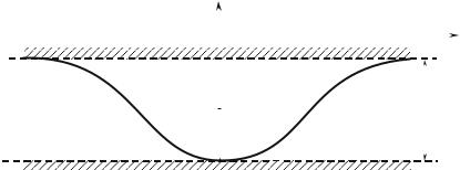
ε(k) = ε0 − 2A cos kd |
(8.20) |
ε(k) is an even function, periodic in k, which describes the totality of its values, i.e. the interval [ε0 −2A, ε0 + 2A], when k varies from −π/d to π/d (Fig. 8.4). The domain of accessible energies ε constitutes an allowed band ; a value of ε chosen outside of the interval [ε0 − 2A, ε0 + 2A] does not correspond to a k- value, it belongs to a forbidden domain. The range −π/d ≤ k < π/d is called “the first Brillouin zone,” a concept introduced in 1930 by Léon Brillouin, a French physicist; it is su cient to study the physics of the problem. Note that
− |
|
ε(k) |
|
|
|
π/d |
|
|||||
|
|
|||||||||||
|
π/d |
|
|
|
k |
|||||||
|
|
|
|
|
|
|
|
|||||
|
|
|
|
|
|
|
|
|||||
|
|
|
ε0 + |
|
2 A |
|
|
|
|
|
||
|
|
|
|
|
|
|
|
|
||||
|
|
|
|
ε0 |
|
|
|
|
4 |
|
A |
|
|
|
|
|
|
|
|
|
|
|
|||
|
|
|
ε |
|
|
|
|
|
|
|
|
|
|
0 − |
|
2 A |
|
|
|
|
|
||||
|
|
|
|
|
|
|
|
|
|
|
|
|
|
|
|
|
|
|
|
|
|
|
|
|
|
Fig. 8.4 : Dispersion relation in the crystal.
in the neighborhood of k = 0, ε(k) ε0 − 2A + Ad2k2 + . . . which looks like the free electron dispersion relation, if an e ective mass m is defined such that 2/2m = Ad2. This mass also expresses the smaller or larger di culty for an electron to move under the application of an external electric field, due to the interactions inside the solid it is subjected to.
The wave function associated with ε(k) is given by
|
+∞ |
|
ψk (x) = |
exp iknd · φ0(x − nd) |
(8.21) |
|
n=−∞ |
|
The Eigenstates for the Chosen Model |
183 |
This expression can be transformed into
ψk (x) = exp ikx · |
+∞ |
|
exp −ik(x − nd) · φ0(x − nd) |
(8.22) |
|
|
n=−∞ |
|
which is the product of a plane wave by a periodic function uk (x), of period d : indeed, for n integer,
|
+∞ |
uk (x + n d) = |
exp −ik(x + n d − nd) · φ0(x + n d − nd) |
n=−∞
+∞
(8.23)
=exp −ik(x − n d) · φ0(x − n d) = uk(x)
n =−∞
This type of solution of the Schroedinger stationary equation
ψk (x) = eikx · uk(x) |
(8.24) |
can be generalized, for a three-dimensional periodic potential V (r), into
|
|
ψk (r) = eik·r · uk |
(8.25) |
This is the so-called Bloch function, from the name of Felix Bloch, who, in his doctoral thesis prepared in Leipzig under the supervision of Werner Heisenberg and defended in July 1928, was the first to obtain the expression of a crystal wave function, using a method analogous to the one followed here. The expression results from the particular form of the di erential equation to be solved (second derivative and periodic potential) and is justified using the Floquet theorem.
Expression (8.21) of ψk (x), established in the case of weak coupling between neighboring atomic sites, can be interpreted as a Linear Combination of Atomic Orbitals (LCAO), since the φ0’s then do not di er much from the atomic solutions ϕ. This model is also called “tight binding” as it privileges the atomic states. When the atomic states of two neighboring sites are taken as orthogonal, this is the so-called “Hückel model.”
The ψk (x) functions are delocalized all over the crystal. The extreme energy states, at the edges of the energy band, correspond to particular Bloch functions : the minimum energy state ε0 − 2A is associated with ψ0(x) =
|
+∞ |
φ (x |
− |
nd), the addition in phase of each localized wave function : this |
||||
|
n=−∞ |
0 |
|
|
|
+ |
|
|
is a situation comparable to the bonding symmetrical state of the H |
2 |
ion; the |
||||||
|
|
|
|
|
+∞ |
n |
||
state of energy ε0 + 2A is associated with ψπ/d(x) = |
n=−∞(−1) φ0 |
(x−nd), |
||||||
alternate addition of each localized wave function and is analogous to the antibonding state of the H+2 ion.