

Statistical physics (2005)
.pdf270 |
Solution of the Exercises and Problems |
|
4 |
|
|
|
|
|
|
|
|
|
|
|
|
3 |
|
|
|
|
|
|
|
|
|
|
|
D(E) |
2 |
|
|
|
|
|
|
|
|
|
|
|
|
|
|
|
|
|
|
|
|
|
|
|
|
|
1 |
|
|
|
|
|
|
|
|
|
|
|
|
0 |
0 |
1 |
2 |
3 |
4 |
5 |
6 |
7 |
8 |
9 |
10 |
|
1 |
|||||||||||
|
|
|
|
|
|
|
E |
|
|
|
|
|
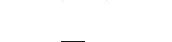
Fig. 2: Densities of states D+/D0 (lower curve) and D−/D0 (upper curve), plotted versus / 0.
II.3.
(a) For the branch = E−(k),
E−(k) = 2(k − k0)2 − 0
2m
the variation of which is given in Fig.1. The spectrum of the permitted energies is [− 0, ∞].
– For − 0 < ≤ 0, there are two possible wavevector moduli k for a given energy :
…
2m
k1,2 = k0 ± 2 ( + 0)
– For > 0, there is a single allowed wavevector modulus :
…
2m
k = k0 + 2 ( + 0)
(b) One then deduces, for > 0
Å … 0 ã
D−( ) = D0( ) 1 +
+ 0
and for < 0 (adding both contributions corresponding for either sign in the k1,2 formula) :
… 0
D−( ) = 2D0( )
+ 0
Problem 2002 : Physical Foundations of Spintronics |
271 |
The corresponding curve is plotted in Fig. 2.
II.4.
(a)Assume that the electrons are accommodated one next to the other in the available energy levels. Since the temperature is taken to be zero, the first electron must be located on the fundamental level, the second one on the first excited level, and so forth. Thus the first levels to be
filled are those of the E− branch, with k around k0, the Fermi energy F being a little larger than − 0 for N small. When N increases, the energyF also increases. It reaches 0 when all the states of the E− branch, of wave vectors ranging between 0 and 2k0, are filled. For larger numbers of electrons, both branches E± are filled.
(b)The E+ branch remains empty until F reaches the value F = 0. There are then
|
0 |
|
|
|
|
π 2 |
0 |
|
|
N = − 0 D−( )d = |
|||||||
|
|
|
|
|
|
2LxLym |
|
|
electrons on the E− branch. |
|
|
|
|
|
E−(k) < F , i.e., |
||
(c) In |
the E− branch, the filled |
states |
verify |
|||||
k1 |
< k < k2 with : |
|
|
|
|
|
|
|
|
|
|
|
|
|
|
||
|
k1,2 = k0 ± |
… |
|
2 ( F + 0) |
|
|
||
|
|
|
|
2m |
|
|
|
|
(see the dashed lines in Fig.1). The extremities of the corresponding k vectors are thus located inside a ring, limited by two Fermi “surfaces” consisting of the circles of respective radii k1 and k2.
II.5.
(a)When N is larger than N , one has to add the extra N − N electrons in both branches, up to the Fermi level. The situation is then given by
the dotted line in Fig.1. For either E± branch, the extremities of the
wave vectors k corresponding to the filled states are located inside the disk defined by E±(k) < F .
(b)For the E+ (resp. E−) branch, the radius of the disk corresponding to the occupied states is determined by E+(kF+) = F (resp. E−(kF−) = F ), with :
kF± = k0 |
+ |
… |
|
2 ( F + 0) |
|
|
|
|
|
2m |
|
In either branch, the Fermi “surface” is a circle for this two-dimensional problem.
(c) One finds :
N − N = 0 |
F |
(D+( ) + D−( )) d = π 2 |
F |
|
|
|
|
LxLym |
|

272 |
Solution of the Exercises and Problems |
One then deduces the relation between the electrons number and the Fermi energy :
N = |
LxLym |
(2 0 + F ) |
|
π 2 |
|||
|
|
II.6.
(a)The energies E±(B) in either branch only vary to second order in B, i.e., one has E±(B) = E±0 + O(B2). This implies that the Fermi energy too only varies to second order in B.
(b)The total magnetization at zero temperature is the sum of the average
ˆ
values of Sz in each filled quantum state, i.e.,
M = |
|
|
(B) ˆ |
(B) |
|
(B) |
ˆ |
(B) |
|
||||||||
|
Ψk,+|Sz |Ψk,+ + |
Ψk,−|Sz |Ψk,− |
|||||||||||||||
|
k<kF+ |
|
|
|
|
|
|
k<kF− |
|
|
|
|
|
|
|
|
|
= |
|
k+ |
|
4αk |
2π |
kdk + 0 |
k− |
|
|
2π |
kdk |
||||||
− 0 |
|
|
|
4αk |
|||||||||||||
|
|
F |
γB LxLy |
|
|
F γB LxLy |
|
||||||||||
One thus finds : |
|
|
|
|
|
|
|
|
|
|
|
|
|
|
|
|
|
M = |
γB LxLy |
(kF− − kF+) = |
LxLy |
γBm |
|
||||||||||||
4α |
|
|
2π |
4π |
|
||||||||||||
II.7. One returns to the expression of question I.4, replacing a±(0) by a±(tn) and a±(t) by a±(tn+1). One averages over the angle φn, using the fact that this angle is not correlated to a±(tn) : a+(tn) a−(tn) e−iφn = 0. One thus finds that the term in sin(2ωτ ) does not contribute and then gets the relation given in the text : s¯(tn+1) = cos(2ωτ ) s¯(tn).
II.8.
(a)If ωτ 1, then cos(2ωτ ) 1 − 2ω2τ 2. The change of s¯(t) in a time interval τ between two collisions is then weak.
(b) In the |
time |
interval |
t τ , |
the |
number |
of |
collisions |
n = t/τ |
1 takes place (the fact that t is not an exact multiple of |
||||||
τ plays a negligible role). Consequently, |
|
|
|
|
|||
|
s¯(t) = s¯(0) (cos(2ωτ ))n = s¯(0) exp (n ln(cos(2ωτ ))) |
|
|||||
Using ln(cos(2ωτ )) |
ln(1 − 2ω2τ 2) |
|
−2ω2τ 2, |
one |
obtains |
||
s¯(t) = s¯(0) e−t/td |
with td = 1/(2ω2τ ). |
|
|
|
|
||
(c)The shorter τ , the longer td. Paradoxically, a poor conductor, in which the time interval between collisions is very short, leads to a longer spin relaxation time than a good conductor. This surprising result can be put together with the quantum Zenon e ect, in which one finds that a frequent observation of a system prevents its evolution.
Problem 2002 : Physical Foundations of Spintronics |
273 |
(d)One finds ω = 7.6 × 10⁹ sec−1 and td = 8.7 × 10⁻⁹ sec. As announced in the introduction of the text, the spin relaxation time td can be much longer than the interval τ between collisions, corresponding to the relaxation time of the electron velocity.
II.9. Let us write the rate equation for the spins + and − populations :
df+ |
= g+ − |
f+ |
− |
f+ |
+ |
f− |
|
df− |
= g− − |
f− |
− |
f− |
+ |
f+ |
dt |
tr |
td |
td |
|
dt |
tr |
td |
td |
In steady-state regime, one has df+/dt = df−/dt = 0, which leads to
1 |
1 |
|
ã |
1 |
|
|
|
|
1 |
1 |
|
ã |
1 |
|
|||||||||||||||||||
|
|
|
+ |
|
|
g+ + |
|
|
g− |
|
|
|
|
|
|
|
|
+ |
|
|
g− + |
|
|
g+ |
|||||||||
f+ = |
Å tr |
t |
t |
|
|
|
= |
|
Å |
t |
|
t |
t |
|
|||||||||||||||||||
|
1d |
2 |
|
|
d |
|
f− |
|
|
r |
|
1d |
2 |
|
|
d |
|||||||||||||||||
|
|
|
|
|
|
|
|||||||||||||||||||||||||||
|
|
|
|
|
+ |
|
|
|
|
|
|
|
|
|
|
|
|
|
|
|
+ |
|
|
|
|
||||||||
|
|
|
|
tr 2 |
tr td |
|
|
|
|
|
|
|
|
|
|
|
tr 2 |
tr td |
|
|
|||||||||||||
and thus |
|
|
|
|
|
|
|
|
|
|
|
|
|
|
|
|
|
|
|
|
|
|
|
|
|
|
|
|
|
|
|
||
|
|
|
|
|
|
|
|
|
P = |
g+ − g− |
|
1 |
|
|
|
|
|
|
|
|
|
|
|
|
|
|
|
|
|
||||
|
|
|
|
|
|
|
|
|
g+ + g− 1 + 2 |
tr |
|
|
|
|
|
|
|
|
|
|
|
|
|
|
|
||||||||
|
|
|
|
|
|
|
|
|
|
|
|
|
|
|
|
|
|
|
|
|
|
|
|
|
|
|
|||||||
|
|
|
|
|
|
|
|
|
|
|
|
|
|
td |
|
|
|
|
|
|
|
|
|
|
|
|
|||||||
|
|
|
|
|
|
|
|
|
|
|
|
|
|
|
|
|
|
|
|
|
|
|
|
|
|
|
|
|
|
||||
To maintain a high polarization, at fixed injection rate, one must minimize the denominator, and thus select a material in which td is as large as possible, consequently in which collisions occur very frequently. Examples of these developments, together with references, may be found in the paper in Physics Today volume 52 (1999) p.33.