

Statistical physics (2005)
.pdf132 |
Chapter 6. General Properties of the Quantum Statistics |
In §6.1, we will show how the statistical properties of indistinguishable independent particles are more conveniently described in the grand canonical ensemble. In §6.2 we will explain how the grand canonical partition function ZG is factorized into terms, each one corresponding to a one-particle quantum state. In §6.3 the Fermi-Dirac and the Bose-Einstein distributions will be deduced, which give the average number of particles of the system occupying a quantum state of given energy at temperature T , and the associated thermodynamical potential, the grand potential, will be expressed.
The §6.4 will be a (long) Quantum Mechanics parenthesis, it will be shown there that a macroscopic system, with extremely close energy levels, is conveniently described by a density of states, that will be calculated for a free particle. In §6.5, this density of states will be used to obtain the average value, at fixed temperature, of physical parameters in the case of indistinguishable particles. Finally, in §6.6, the criterion used in §4.3 to define the domain of Classical Statistics will be justified and it will be shown that the Maxwell-Boltzmann Classical Statistics is the common limit of both Quantum Statistics when the density decreases or the temperature increases.
6.1Use of the Grand Canonical Ensemble
In chapter 5 we learnt the properties requested for the wave function of N indistinguishable particles, when these particles are fermions or when they are bosons. (From the present chapter until the end of the book, the study will be limited to indistinguishable and independent particles.) Now we look for the statistical description of such a system in thermal equilibrium at temperature T and first show, on the example of two particles, that the use of the canonical ensemble is not convenient.
6.1.1Two Indistinguishable Particles in Thermal Equilibrium : Statistical Description
in the Canonical Ensemble
Consider a system of two indistinguishable particles. The one-particle energy levels are noted ε1, . . . , εk , . . . , and are assumed to be nondegenerate (a degenerate level is described by several states at the same energy but with di erent indexes). The canonical partition function for a single particle at temperature T is written :
1 |
|
|
Z1 = e−βεk with β = |
|
(6.1) |
kB T |
||
k |
|
|
Use of the Grand Canonical Ensemble |
133 |
Now consider the two particles. For a given microscopic configuration, the total energy is εi + εj . After having recalled the results for two distinguishable particles, we will have to separately consider the case of fermions and that of bosons.
We have seen in §2.4.5 that for distinguishable particles |
|
Z2disc = (Z1)2 |
(6.2) |
since there is no limitation to the levels occupation by the second particle.
Fermions cannot be more than one to occupy the same state. Consequently, as soon as the level of energy εi is occupied by the first particle, the second one cannot be on it. Thus
|
|
1 |
|
|
|
|
|
|
|
Z2fermions = |
|
e−β(εi |
+εj ) = e−β(εi+εj ) |
(6.3) |
|
|
|
2 |
|||||
|
|
|
|
i=j |
|
i<j |
|
Let us compare Z2fermions to (Z1)2 : |
|
|
|
||||
(Z1)2 |
= i |
e−βεi j |
e−βεj = |
i |
e−β2εi + 2 i<j e−β(εi+εj ) |
(6.4) |
|
(Z1)2 |
= e−β2εi + 2Z2fermions |
|
|
(6.5) |
|||
|
i |
|
|
|
|
|
|
In the case of bosons, in addition to the configurations possible for the fermions, the two particles can also lie on the same level :
Z2bosons = |
e−β(εi+εj ) |
(6.6) |
|||
|
i≤j |
|
|
|
|
Let us relate (Z1)2 to Z2bosons : |
|
|
|
|
|
(Z1)2 |
= Z2bosons + |
1 |
e−β |
(εi+εj ) |
(6.7) |
|
|||||
2 |
|||||
|
|
|
i=j |
|
|
(Z1)2 |
= Z2bosons + Z2fermions |
|
(6.8) |
||
It was easy to determine the levels available for the particles in this example because they were only two. For three particles one must then consider which restrictions appear for the third one because of the levels occupied by the first two particles. For N particles one should again proceed step by step, but this method is no longer realistic!
6.1.2Description in the Grand Canonical Ensemble
To avoid complicated conditions on the occupation numbers nk one will work in the grand canonical ensemble, assuming in a first step that the total number

134 Chapter 6. General Properties of the Quantum Statistics
of particles of the system is arbitrary. Thus one will calculate ZG and the grand potential A ; then the value of the Lagrange parameter α = βµ (or that of the chemical potential µ) will be fixed in such a way that the average number of particles N , deduced from the statistical calculation, coincides with the
real number of particles in the system. We know (§2.5.4) that the relative
√
fluctuation on N introduced by this procedure is of the order of 1/ N , that is, of the order of a few 10−12 for N of the order of the Avogadro number.
6.2Factorization of the Grand Partition Function
6.2.1Fermions and Bosons
By definition
∞ |
∞ |
|
ZG(α, β) = eαN ZN (β) = |
eβµN ZN (β) |
(6.9) |
N =0 |
N =0 |
|
where N is one of the numbers of particles and where α and the chemical potential are related by α = βµ. The canonical partition function ZN (β) corresponding to N particles is given by
ZN (β) = e−βEn |
(6.10) |
n |
|
Let us introduce the occupation numbers nk of the quantum states εk :
ZG = N =0e |
|
Ñ |
n =Ne |
|
é |
(6.11) |
∞ |
βµ |
nk |
|
−β |
nk εk |
|
|
k |
|
|
k |
|
|
k
with
nk = N |
(6.12) |
k
and the energy for this configuration of the N particles being given by
nk εk = EN |
(6.13) |
k
Factorization of the Grand Partition Function |
135 |
As the sum is performed over all the total numbers N and all the particle
distributions in the system, ZG is also written |
|
|
|||
ZG = |
e |
|
|
(6.14) |
|
|
|
βµ |
nk −β |
|
nk εk |
|
|
|
k |
k |
|
= |
{|n1...nk >} |
|
|
(6.15) |
|
e |
|
||||
|
|
β |
nk (µ−εk ) |
|
|
k
{|n1...nk >}
In the latter expression, one separates the contribution of the state ε1 : this is the term
eβ(µ−ε1 )n1 |
(6.16) |
n1
which multiplies the sum concerning all the other states, with n1 taking all possible values. One then proceeds state after state, so that ZG is written as a product of factors :
ZG = ∞ |
|
eβ(µ−εk )nk |
(6.17) |
k |
n |
k |
|
=1 |
|
|
Each factor concerns a single state εk and its value depends on the number of particles which can be located in this state, i.e., of the nature, fermions or bosons, of the considered particles. Note that, since ZG is a product of factors, ln ZG is a sum of terms, each concerning a one-particle state of the type εk .
6.2.2Fermions
In this case, the quantum state εk is occupied by 0 or 1 particle : there are only two terms in nk , the contribution of the state εk in ZG is the factor
1 + exp β(µ − εk), whence
∞ |
|
k |
(6.18) |
ZG fermions = (1 + eβ(µ−εk )) |
|
=1 |
|
6.2.3Bosons
The state εk can now be occupied by 0, 1, 2,... particles, so that nk varies from zero to infinity. The contribution in ZG of the state εk is thus the factor
∞ |
1 |
|
nk =0eβ(µ−εk )nk = |
|
(6.19) |
1 − eβ(µ−εk ) |

136 |
Chapter 6. General Properties of the Quantum Statistics |
This geometrical series can be summed only if exp(α − βεk ) is smaller than unity, a condition to be fulfilled by all the states εk. One will thus have to verify that µ < ε1, where ε1 is the one-particle quantum state with the lowest energy, i.e., the fundamental state. This condition is also expressed through
α = βµ as α < βε1.
Then the grand partition function takes the form :
∞ |
|
1 |
|
k |
|
|
|
− |
|
|
|
ZG bosons = |
1 eβ(µ−εk ) |
(6.20) |
|
=1 |
|
||
|
|
|
|
6.2.4Chemical Potential and Number of Particles
The grand canonical partition function ZG is associated with the grand potential A such that
A = −kB T ln ZG |
(6.21) |
As specified in §3.5.3, the partial derivatives of the grand partition function provide the entropy, the pressure and the average number of particles N :
dA = −SdT − P dΩ − N dµ |
(6.22) |
In particular the constraint on the total number of particles of the system is expressed from :
N = − Å |
∂A |
ãT,Ω |
(6.23) |
∂µ |
6.3Average Occupation Number; Grand Potential
From the grand partition function ZG one deduces average values at temperature T of physical parameters of the whole system, but also of the state εk . In particular the average value of the occupation number nk of the state of energy εk is obtained through
|
|
|
|
nk nk eβ(µ−εk )nk |
1 |
|
∂ ln Z |
G |
|
|||
|
nk |
|
= |
|
β(µ εk )nk |
= |
|
|
|
|
(6.24) |
|
|
−β |
|
∂εk |
|
||||||||
|
|
e |
− |
|
|
|
||||||
nk

Average Occupation Number; Grand Potential |
137 |
For fermions, the average occupation number, the so-called “Fermi-Dirac distribution,” is given by
1 |
1 |
with α = βµ |
|
||
nk F D = |
|
= |
|
(6.25) |
|
eβ(εk −µ) + 1 |
eβεk −α + 1 |
||||
For bosons, this average number is “the Bose-Einstein” distribution which takes the form
1 |
1 |
|
||
nk BE = |
|
= |
|
(6.26) |
eβ(εk −µ) − 1 |
eβεk −α − 1 |
|||
Note : Remember the sign di erence in the denominator between fermions and bosons! Its essential physical consequences are developed in the next chapters.
The average occupation numbers are related to factors in the grand partition function ZG : indeed one will verify that
1 = 1 + eβ(µ−εk )
1 − nk F D
1
1 + nk BE = 1 − eβ(µ−εk )
which are the respective contributions of the level εk fermions or bosons.
(6.27)
(6.28)
to ZG, in the cases of
These occupation numbers yield the average values, at given temperature, thus at fixed β, of physical parameters.
Thus the average number of particles is related to α and β, which appear in f (ε), through
N = |
nk |
(6.29) |
|
k |
|
The total energy of the system at temperature T is obtained from |
|
|
U = |
εk nk |
(6.30) |
k |
|
|
The grand potential A is expressed, like the ZG factors, versus the occupation numbers of the states of energy εk :
A = +kB T |
ln(1 − nk ) |
fermions |
(6.31) |
|
k |
|
|
A = −kB T |
ln(1 + nk ) |
bosons |
(6.32) |
k

138 |
Chapter 6. General Properties of the Quantum Statistics |
6.4Free Particle in a Box ; Density of States (Quantum Mechanics)
The di erent physical parameters, like the average number of particles N , the internal energy U , the grand potential A, were expressed above as sums of contributions arising from the discrete one-particle levels. Now we will first recall what these states are for a free particle confined within a volume of macroscopic characteristic dimensions, i.e., of the order of a mm or a cm (§6.4.1) : such dimensions are extremely large with respect to atomic distances, so that the characteristic energy splittings are very small (§6.4.1a). The boundary conditions (§6.4.1b) of the wave function imply quantization conditions, that we are going to express in two di erent ways. However, for both quantization conditions the same energy density of states D(ε) is defined (§6.4.2), such that the number of allowed states between energies ε and ε + dε is equal to
D(ε) dε.
6.4.1Quantum States of a Free Particle in a Box
a) Eigenstates
By definition a free particle feels no potential energy (except the one expressing the possible confinement) We first consider that the free particle can move through the entire space. Its hamiltonian is given by
|
ˆ2 |
|
ˆ |
p |
|
h = |
2m |
(6.33) |
We are looking for its stationary states (see a course on Quantum Mechanics) : the eigenstate |ψ and the corresponding energy ε satisfy
|
|
ˆ2 |
|
|
|
|
|
p |
|ψ = ε|ψ |
(6.34) |
|
|
|
2m |
|||
i.e., |
|
|
|
|
|
|
2 |
|
|
||
− |
|
∆ψ(r) = εψ(r) |
(6.35) |
||
2m |
|||||
The time-dependent wave function is then deduced :
Ψ(r, t) = ψ(r) exp(−iεt/ ) |
(6.36) |
It is known that the three space variables separate in eq. (6.35) and that it is enough to solve the one-dimension Schroedinger equation
− |
2 d2ψ(x) |
= εxψ(x) |
(6.37) |
2m dx2 |
Free Particle in a Box; Density of States
which admits two equivalent types of solutions :
i) either
ψ(x) = √1 exp ikxx Lx
with kx > 0, < 0 or zero. The time-dependent wave function
1 |
exp i Åkxx − |
εxt |
ã |
|||
Ψ(x, t) = |
√ |
|
|
|||
|
||||||
Lx |
||||||
139
(6.38)
(6.39)
with εx = |
2k2 |
= ωx is a progressive wave : when the time t increases, |
|
x |
|||
2m |
|||
|
|
a state of given phase propagates toward increasing x’s for kx > 0, toward decreasing x’s for kx < 0 ; the space wave function is a constant for kx = 0.
ii) or
ψ(x) = A cos kxx + B sin kxx |
|
|
(6.40) |
where A and B are constants. |
|
|
|
The time-dependent wave function |
|
|
|
Ψ(x, t) = (A sin kxx + B cos kxx) exp Å−i |
εxt |
ã |
(6.41) |
|
corresponds to the same energy εx or the same pulsation ωx as in (6.39).
The solution of progressive-wave type (6.39) is found again if one chooses
√
A = 1/ Lx, B = iA. For real coe cients A and B, when changing the space origin in x there is indeed separation of the space and time variables in (6.41). Then a state of given space phase does not propagate in time, such a wave is stationary.
At three dimensions the kinetic energy terms along the three coordinates add up in the hamiltonian; the energy is equal to
ε = εx + εy + εz |
(6.42) |
and the wave function is the product of three wave functions, each concerning a single coordinate.
Now we are going to express, through boundary conditions on the wave function, that the particle is confined within the volume Ω. This will yield quantization conditions on the wave vector and the energy.
140 |
Chapter 6. General Properties of the Quantum Statistics |
b) Boundary Conditions
The volume Ω containing the particles has a priori an arbitrary shape. However, it can be understood that each particle in motion is most of the time at a large distance from the container walls, so that the volume properties are not sensitive to the surface properties as soon as the volume is large enough. It is shown, and we will admit it, that the Statistical Physics properties of a macroscopic system are indeed independent of the shape of the volume Ω. For convenience we will now assume that Ω is a box (Lx, Ly , Lz), with macroscopic dimensions of the order of a mm or a cm.
We consider a one-dimension problem, on a segment of length Lx. The presence probability of the particle is zero outside the interval [O, Lx], in the region where the particle cannot be found. There are two ways to express this condition :
i) Stationary boundary conditions :
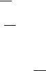
To indicate that the particle cannot leave the interval, one assumes that in x = 0 and x = Lx potential barriers are present, which are infinitely high and thus impossible to overcome. Thus the wave function vanishes outside the interval [O, Lx] and also at the extremities of the segment, to ensure its continuity at these points; since it vanishes at x = 0, it must be of the form ψ(x) = A sin kxx (Fig. 6.1). The cancellation at x = Lx yields
kxLx = nxπ
where nx is an integer, so that
π
kx = nx Lx
The wave vector is an integer multiple of π , it is quantized.
Lx
For such values of kx, the time-dependent wave function is given by
Ψ(x, t) = A sin kxx exp Å−i εxt ã
(6.43)
(6.44)
(6.45)
One understands that the physically distinct allowed values are restricted to nx > 0 : indeed taking nx < 0 is just changing the sign of the wave function, which does not change the physics of the problem. The value nx = 0 is to be rejected since a wave function has to be normalized to unity and thus cannot cancel everywhere. In the same way ky and kz are quantized by the conditions of cancellation of the wave function on the surface : finally the allowed vectors
k for the particle confined within the volume Ω are of the form
k = Ånx |
π |
, ny |
π |
, nz |
π |
ã |
(6.46) |
|
|
|
|||||
Lx |
Ly |
Lz |
Free Particle in a Box; Density of States |
141 |
ψ(x)
x
O 
Lx
Fig. 6.1: The free-particle wave function is zero outside the interval ]O, Lx[.
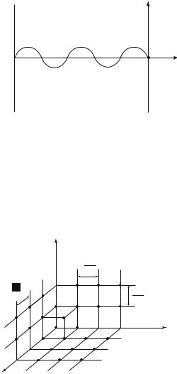
the three integers nx, ny , nz being strictly positive. In the space of the wave vectors (Fig. 6.2), the extremities of these vectors are on a rectangular lattice
defined by |
|
|
|
|
Å |
π |
|
π |
|
π |
|
ã |
|
π3 |
|
π3 |
Lx |
i, |
Ly |
j, |
Lz |
||||||
|
|
the three vectors |
|
|
|
|
|
|
k |
. The unit cell built on these |
|||
vectors is |
|
= |
|
. |
|
|
|
|
|
|
|
|
|
LxLyLz |
Ω |
|
|
|
|
|
|
|
|
||||
|
|
|
kz |
|
|
|
π |
|
|
|
Ly |
π |
|
|
π |
|
L |
x |
|
|
|
||
|
|
Lz |
|
|
|
|
|
|
|
|
ky |
|
kx |
Fig. |
|
6.2: Quantization of the k-space for boundary conditions of the |
stationary-wave type. Only the trihedral for which the three k-components are positive is to be considered.
ii) Periodical boundary [Born-Von Kármán (B-VK)] conditions :
Here again one considers that when a solid is macroscopic, all that deals with its surface has little e ect on its macroscopic physical parameters like its pressure, its temperature. The solid will now be closed on itself (Fig. 6.3) and this will not noticeably modify its properties : one thus suppresses surface