

Statistical physics (2005)
.pdf206 |
Chapter 9. Bosons : Helium 4, Photons, Thermal Radiation |
9.2Bose-Einstein Distribution of Photons
Our daily experience teaches us that a heated body radiates, as is the case for a radiator heating a room or an incandescent lamp illuminating us through its visible radiation. Understanding these mechanisms, a challenge at the end of the 19th century, was at the origin of M. Planck’s quanta hypothesis (1901). For more clarity we will not follow the historical approach but rather use the tools provided by this course. Once the results obtained, we will return to the problems Planck was facing.
9.2.1Description of the Thermal Radiation ; the Photons
Consider a cavity of volume Ω heated at temperature T (for example an oven) and previously evacuated. The material walls of this cavity are made of atoms, the electrons of which are promoted into excited states by the energy from the heat source. During their deexcitation, these electrons radiate energy, under the form of an electromagnetic field which propagates inside the cavity, is absorbed by other electrons associated to other atoms, and so forth, and this process leads to a thermal equilibrium between the walls and the radiation enclosed inside the cavity.
If the cavity walls are perfect reflectors, classical electromagnetism teaches us
that the wave electrical field E is zero inside the perfect conductor and normal
to the wall on the vacuum side (due to the condition that Etangential is conti-
nuous), and that the corresponding magnetic field B must be tangential. In order to produce the resonance of this cavity and to establish stationary waves, the cavity dimension L should contain an integer number of half-wavelengths λ. The wave vector k = 2π/λ and L are then linked.
|
|
|
−ωt) |
An electromagnetic wave, given in complex notation by E(ω, k) exp i(k ·r |
|||
is characterized by its wave vector k and its frequency ω ; it can have two independent polarization states (either linear polarizations along two perpendicular directions, or left or right circular polarizations) on which the direction
|
|
|
|
of the electric field in the plane normal to k is projected. Finally its intensity |
|||
|
|
2 |
. |
is proportional to |E(ω, k)| |
|
||
Since the interpretation of the photoelectric e ect by A. Einstein in 1905, it has been known that the light can be described both in terms of waves and of particles, which are the photons. The quantum description of the electromagnetic field is taught in advanced Quantum Mechanics courses. Here we only specify that the photon is a relativistic particle of zero mass, so that

Bose-Einstein Distribution of Photons |
207 |
the general relativistic relation between the energy ε and the momentum p,
ε = p2c2 + m20c4, where c is the light velocity in vacuum, reduces in this case to ε = pc. Although the photon spin is equal to 1, due to its zero mass it only has two distinct spin states. The set of data consisting in p and the photon spin value defines a mode.
The wave parameters k and ω and the photon parameters are related through the Planck constant, as summarized in this table :
electromagnetic wave |
particle : photon |
||
|
|
|
|
wave vector k |
|
p = k momentum |
|
frequency ω |
|
ε = ω energy |
|
|
2 |
|
|
intensity |E(k, ω)| |
number of photons |
||
|
|||
polarization (2 states) |
spin (2 values) |
||
|
|
|
|
Let us return to the cavity in thermal equilibrium with the radiation it contains : its dimensions, in Ω1/3, are very large with respect to the wavelength of the considered radiation. The exact surface conditions do not matter much : as in the particles case (see § 6.4.1b) ), rather than using the stationary wave conditions, we prefer the periodic limit conditions (“Born-Von Kármán” conditions) : in a thought experiment we close the system on itself, which
quantizes k and consequently, p and the energy. Assuming the cavity is a box of dimensions Lx, Ly, Lz , one obtains :
k = (kx, ky , kz ) = 2π Å |
nx |
, |
ny |
, |
nz |
ã |
(9.24) |
Lx |
Ly |
Lz |
where nx, ny, nz are positive or negative integers, or zero.
Then
p = h Å |
nx |
, |
ny |
, |
nz |
ã |
(9.25) |
Lx |
Ly |
Lz |
|||||
ε = pc = ω = hν |
|
(9.26) |
|||||
9.2.2Statistics of Photons, Bosons in Non-Conserved Number
In the photon emission and absorption processes of the wall atoms, the number of photons varies, and there are more photons when the walls are hotter : in this system the constraint on the conservation of particles number, that existed in §9.1, is lifted. This constraint was defining the chemical potential µ as a Lagrange multiplier, which no longer appears in the probability law for photons, i.e., the chemical potential is zero for photons.

208 |
Chapter 9. Bosons : Helium 4, Photons, Thermal Radiation |
Let us consider the special case where only a single photon mode is possible, i.e., a single value of p, of the polarization and of ε in the cavity at thermal equilibrium at temperature T . Any number of photons is possible, thus the partition function z(ε) is equal to
∞ |
1 |
|
z(ε) = n=0 e−βnε = |
|
(9.27) |
1 − e−βε |
and the average energy at T of the photons in this mode is given by
n ε = − |
1 ∂z(ε) |
= |
ε |
||||
z(ε) |
|
∂β |
|
eβε − 1 |
|
||
For the occupation factor of this mode, one finds again the Bose-Einstein distribution in which µ = 0, i.e.
f (ε) = |
1 |
(9.28) |
eβε − 1 |
[Note that in the study of the specific heat of solids (see §2.4.5) a factor similar to (9.28) appeared : in the Einstein and Debye models the quantized solid vibrations are described by harmonic oscillators. Changing the vibration
state of the solid from n + 1 |
|
ω to |
n + 1 |
+ 1 ω is equivalent to creating |
|
a quasi-particle, called a |
2 |
|
|
2 |
|
phonon, which follows the Bose-Einstein statistics. |
|||||
|
|
|
|
|
|
The number of phonons is not conserved].
If now one accounts for all the photons modes, for a macroscopic cavity volume
|
|
|
|
|
|
|
|
|
|
Ω, one can define the densities of states D (k), Dp(p), D(ε) such that the |
|||||||||
|
|
|
|
|
k |
|
|
|
|
|
|
|
|
|
|
|
|
|
|
number dn of modes with a wave vector between k and k + dk is equal to dn : |
|||||||||
|
Ω |
3 |
|
3 |
|
|
|||
|
|
|
|
|
|
||||
dn = 2 · |
(2π)3 |
d k = Dk(k)d k |
|
||||||
|
Ω |
|
|
|
|
|
|||
dn = 2 · |
|
d3p = Dp(p)d3p |
|
|
|
||||
h3 |
|
|
|
||||||
that is, |
|
|
|
|
|
|
|
|
|
|
Ω |
|
|
2Ω |
|
||||
D (k) = |
|
|
|
, |
Dp(p) = |
|
|
(9.29) |
|
4π3 |
h3 |
||||||||
k |
|
|
|
||||||
The factor 2 expresses the two possible values of the spin of a photon of fixed
k (or p).
Since the energy ε only depends of the modulus p, one obtains D(ε) from
D(ε)dε = 2 |
Ω |
4πp2dp = 8π |
Ω |
ε2dε |
||
|
h3c3 |
|||||
|
|
h3 |
|
(9.30) |
||
|
8πΩ |
|
|
|||
D(ε) = |
ε2 |
|
|
|||
h3c3 |
|
|
||||
|
|
|
|
|||

Bose-Einstein Distribution of Photons |
209 |
In this “large volume limit”, one can express the thermodynamical parameters.
The thermodynamical potential to be considered here is the free energy F (since µ = 0)
F = −kB T ln Z = kB T 0 |
∞ ln(1 − e−βε)D(ε)dε |
(9.31) |
||||||||||||||
The internal energy is written |
|
|
|
|
|
|
|
|
|
|||||||
U = 0∞ εD(ε)f (ε)dε |
|
∞ |
|
8πΩ hν3dν |
(9.32) |
|||||||||||
∞ 8πΩ ε3 |
|
|
|
|||||||||||||
= 0 |
|
|
|
|
dε = |
0 |
|
|
|
|
|
|
|
|||
h3c3 |
eβε − 1 |
|
c3 |
eβhν − 1 |
|
|||||||||||
i.e., |
|
|
|
|
|
|
|
|
|
|||||||
|
U = 0∞ Ωu(ν)dν |
|
|
|
|
|
|
|
||||||||
with |
|
|
|
|
|
|
|
|
|
|||||||
|
u(ν) = |
8πh |
|
|
|
ν3 |
|
|
|
|
|
|
(9.33) |
|||
|
c3 eβhν − |
1 |
|
|
|
|
||||||||||
|
|
|
|
|
|
|
|
|
||||||||
The photon spectral density in energy u(ν) is defined from the energy contribution dU of the photons present inside the volume Ω, with a frequency between
ν and ν + dν :
dU = Ωu(ν)dν |
(9.34) |
The expression (9.33) of u(ν) is called the Planck law.
The total energy for the whole spectrum is given by |
|
|||||
U = |
8πΩ |
(kB T )4 |
0 |
∞ x3dx |
(9.35) |
|
h3c3 |
|
ex − 1 |
||||
where the dimensionless integral is equal to Γ(4)ζ(4) with Γ(4) = 3! and
ζ(4) = π4 (see the section “Some useful formulae” in this book). Introducing
90
= h/2π, the total energy becomes
U = |
π2 |
Ω |
(kB T )4 |
(9.36) |
|
15 |
( c)3 |
||||
|
|
|
The free energy U and the internal energy F are easily related : in the integration by parts of (9.31), the derivation of the logarithm introduces

210 |
Chapter 9. Bosons : Helium 4, Photons, Thermal Radiation |
the Bose-Einstein distribution, the integration of D(ε) provides a term in ε3/3 = ε . ε2/3. This exactly gives
F = −U = −π2 Ω (kB T )4
3 45 ( c)3
[to be compared to (9.11), which is valid for material particles with a density of states in ε1/2, whereas the photons density varies in ε2]. Since
|
|
|
dF = −SdT − P dΩ |
|
|
(9.37) |
||||||||
one deduces |
|
|
|
|
|
|
|
|
|
|
|
|
|
|
S = − Å |
∂F |
ãΩ |
|
4π2 |
Å |
kB T |
ã |
3 |
||||||
|
|
|||||||||||||
|
= |
|
|
|
kB Ω |
|
(9.38) |
|||||||
∂T |
45 |
c |
||||||||||||
P = − Å |
∂F |
ãT |
= − |
F |
|
|
|
(9.39) |
||||||
|
|
|
|
|
|
|||||||||
∂Ω |
Ω |
|
|
|
||||||||||
P = |
π2 (kB T )4 |
|
|
|
|
|
|
|
|
(9.40) |
||||
45 |
|
|
( c)3 |
|
|
|
|
|
|
|
|
|||
|
|
|
|
|
|
|
|
|
|
|
|
|||
The pressure P created by the photons is called the radiation pressure.
9.2.3Black Body Definition and Spectrum
The results obtained above are valid for a closed cavity, in which a measurement is strictly impossible because there is no access for a sensor. One is easily convinced that drilling a small hole into the cavity will not perturb the photons distribution but will permit measurements of the enclosed thermal radiation, through the observation of the radiation emitted by the hole. Besides any radiation coming from outside and passing through this hole will be trapped inside the cavity and will only get out after thermalization. This system is thus a perfect absorber, whence its name of black body.
In addition we considered that thermal equilibrium at temperature T is reached between the photons and the cavity. In such a system, at steady-state, for each frequency interval dν, the energy absorbed by the walls exactly balances their emitted energy, which is found in the photon gas in this frequency range, that is, Ωu(ν)dν. Therefore the parameters we obtained previously for the photon gas are also those characterizing the thermal emission from matter at temperature T , whether this emission takes place in a cavity or not, whether this matter is in contact with vacuum or not. We will then be able to compare the laws already stated, and in the first place the Planck law, to experiments performed on thermal radiation.
Bose-Einstein Distribution of Photons |
211 |
The expression (9.33) of u(ν) provides the spectral distribution of the thermal radiation versus the parameter β, i.e. versus the temperature T . For any T , u(ν) vanishes for ν = 0 and tends to zero when ν tends to infinity. The variable is in fact βhν and one finds that the maximum of u(ν) is reached for βhνmax = 2.82, that is,
νmax = 2.82 |
kB T |
(9.41) |
|
h |
|||
|
|
Relation (9.41) constitutes the Wien law.
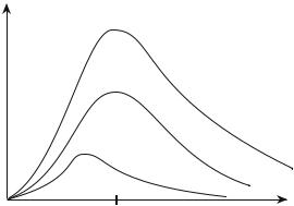
When T increases, the frequency of the maximum increases and for T1 < T2 the whole curve u(ν) for T2 is above that for T1 (Fig. 9.1).
u(ν)
J.s.m−3
5.10−15
T1 < T2 < T3
|
T |
= |
|
|
T |
3 |
6000 |
|
|
|
|
|||
2 |
|
|
K |
|
|
|
|
||
|
|
|
|
T1
|
|
ν |
0 |
4 |
1014Hz |
Fig. 9.1: Spectral density in energy of the thermal radiation for several temperatures.
For small values of ν, u(ν) kB T · |
|
8π |
ν2 |
(9.42) |
||
|
c3 |
|||||
for ν large, u(ν) |
8πh |
ν |
3e−βhν |
(9.43) |
||
c3 |
||||||
At the end of the 19th century, photometric measures allowed one to obtain the u(ν) curves with a high accuracy. Using the then available MaxwellBoltzmann statistics, Lord Rayleigh and James Jeans had predicted that the average at temperature T of the energy of oscillators should take the form (9.42), in kB T ν2. If this latter law does describe the low-frequency behavior of the thermal radiation, it predicted an “ultraviolet catastrophe” [u(ν) would be an increasing function of ν, thus the U V and X emissions should be huge]. Besides, theoretical laws had been obtained by Wilhem Wien and experimentally confirmed by Friedrich Paschen : an exponential behavior at
212 |
Chapter 9. Bosons : Helium 4, Photons, Thermal Radiation |
high frequency like in (9.43) and the law (9.41) of the displacement of the distribution maximum. It was the contribution of Max Planck in 1900 to guess the expression (9.33) of u(ν), assuming that the exchanges of energy between matter and radiation can only occur through discrete quantities, the quanta. Note that the ideas only slowly clarified until the advent in the mid 1920’s of Quantum Mechanics, such as we know it now. It it remarkable that the paper by Bose, proposing the now called “Bose-Einstein statistics,” preceded by a few months the formulation by Erwin Schroedinger of its equation!
The universe is immersed within an infrared radiation, studied in cosmology, the distribution of which very accurately follows a Planck law for T = 2.7 K. It is in fact a “fossil” radiation resulting from the cooling, by adiabatic expansion of the universe, of a thermal radiation at a temperature of 3000 K which was prevailing billions of years ago : according to expression (9.38) of the entropy, an adiabatic process maintains the product ΩT 3. The universe radius has thus increased of a factor 1000 during this period.
The sun is emitting toward us radiation with a maximum in the very near infrared, corresponding to T close to 6000 K. A “halogen” bulb lamp is emitting a radiation corresponding to the temperature of its tungsten filament (around 3000 K), which is immersed in a halogen gas to prevent its evaporation. We ourselves are emitting radiation with a maximum in the far infrared, corresponding to our temperature close to 300 K.
9.2.4Microscopic Interpretation of the Bose-Einstein Distribution of Photons
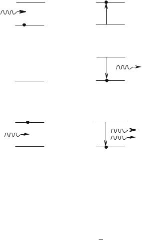
Another schematic way to obtain the Bose-Einstein distribution, and consequently, the Planck law, consists in considering that the walls of the container are made of atoms with only two possible energy levels ε0 and ε1 separated by ε1 − ε0 = hν, and in assuming that the combined system (atoms-photons of energy hν) is at thermal equilibrium (Fig. 9.2). It is possible to rigorously calculate the transition probabilities between ε0 and ε1 (absorption), or between ε1 and ε0 (emission) under the e ect of photons of energy hν. This is done in advanced Quantum Mechanics courses. Here we will limit ourselves to a more qualitative argument, admitting that in Quantum Mechanics a transition is expressed by a matrix element, which is the product of a term 1|V |0 specific of the atoms with another term due to the photons. Besides, we will admit that an assembly of n photons of energy hν is described by a harmonic oscillator, with energy levels splitting equal to hν, lying in the state |n .
The initial state contains N0 atoms in the fundamental state, N1 atoms in the state ε1, and n photons of energy hν.
Bose-Einstein Distribution of Photons
|
BEFORE |
N1 |
E1 |
hν |
|
N0 |
E0 |
N1  E1
E1
N0 |
E0 |
N1 |
E1 |
hν |
|
N0 |
E0 |
213
AFTER
N1 + 1
absorption
N0 − 1
N1 − 1 |
spontaneous |
|
hν |
|
|
N0 + |
1 |
emission |
N1 − 1
induced
hν
emission
N0 + 1
Fig. 9.2: Absorption, spontaneous and induced emission processes for an assembly of two-level atoms in thermal equilibrium with photons.
In the absorption process (Fig. 9.2 top), the number of atoms in the state of energy ε0 becomes N0 − 1, while N1 changes to N1 + 1 ; a photon is utilized, thus the photons assembly shifts from |n to |n − 1 . This is equivalent to considering the action on the state |n of the photon annihilation operator, i.e., according to the Quantum Mechanics course,
√ |
(9.44) |
a|n = n |n − 1 |
The absorption probability per unit time P is proportional to the number of atoms N0 capable of absorbing a photon, to the square of the matrix element appearing in the transition, and is equal, to a multiplicative constant, to :
Pa = N0 |
| 1|V |0 |2 |
| n − 1|a|n |2 |
(9.45) |
= N0 |
| 1|V |0 |2 |
n |
(9.46) |
This probability is, as expected, proportional to the number n of present photons.

214 Chapter 9. Bosons : Helium 4, Photons, Thermal Radiation
In the emission process (Figs. 9.2 middle and bottom), using a similar argument, since the number of photons is changed from n to n + 1, one considers the action on the state |n of the photon creation operator :
a |
+ |
|n = |
√ |
|
|
(9.47) |
|
||||||
|
n + 1 |n + 1 |
|||||
The emission probability per unit time Pe is proportional to the number of atoms N1 that can emit a photon, to the square of the matrix element of this transition and is given by
Pe = N1 |
| 0|V |1 |2 |
| n + 1|a+|n |2 |
(9.48) |
= N1 |
| 0|V |1 |2 |
(n + 1) |
(9.49) |
We find here that Pe is not zero even when n = 0 ( spontaneous emission), but that the presence of photons increases Pe (induced or stimulated emission) : another way to express this property is to say that the presence of photons “stimulates” the emission of other photons. The induced emission was introduced by A. Einstein in 1916 and is at the origin of the laser e ect. Remember that the name “laser” stands for Light Amplification by Stimulated Emission of Radiation.
In equilibrium at the temperature T , n photons of energy hν are present : the absorption and emission processes exactly compensate, thus
N0 |
|
= N1( |
|
+ 1) |
(9.50) |
n |
n |
Besides, for the atoms in equilibrium at allows one to write
N1 = e
N0
One then deduces the value of n
T , the Maxwell-Boltzmann statistics
−βhν |
(9.51) |
1 |
|
n = eβhν − 1 |
(9.52) |
which is indeed the Bose-Einstein distribution of photons. This yields u(ν, T ) through the same calculation of the photons modes as above [formulae (9.29) to (9.33)].
This approach, which is based on advanced Quantum Mechanical results, has the advantage of introducing the stimulated emission concept and the description of an equilibrium from a balance between two phenomena.
9.2.5Photometric Measurements : Definitions
We saw that a “black body” is emitting radiation corresponding to the thermal equilibrium in the cavity at the temperature T . A few simple geometrical
Bose-Einstein Distribution of Photons |
215 |
considerations allow us to relate the total power emitted by a black body to its temperature and to introduce the luminance, which expresses the “color” of a heated body : we will then be able to justify that all black bodies at the same given temperature T are characterized by the same physical parameter and thus that one can speak of THE black body.
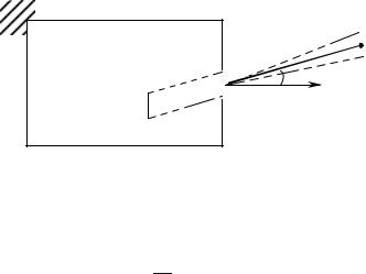
Let us first calculate the total power P emitted through the black-body aperture in the half-space outside the cavity. We consider the photons of frequency ν, to dν, which travel through the aperture of surface dS and have a velocity directed toward the angle θ to dω with the normal n to dS. The number of these photons which pass the hole during dt are included in a cylinder of basis dS and height c cos θdt (Fig. 9.3). They carry an energy

 dω
dω
 θ
θ
n
dS  cdt
cdt
Fig. 9.3: Radiation emitted through an aperture of surface dS in a cone dω around the direction θ.
d2P · dt = |
dω |
|
4π c cos θ dt dS u(ν)dν |
(9.53) |
The total power P radiated into the half-space, by unit time, through a hole of unit surface is given by
|
|
|
π |
|
|
|
|
2π dϕ |
∞ |
|
||
2 |
|
|
|
|
|
|||||||
P = 0 |
cos θ sin θdθ 0 |
|
0 |
c u(ν, T )dν |
(9.54) |
|||||||
4π |
||||||||||||
P = |
c |
|
U |
= |
π2 |
|
(kB T )4 |
= σT 4 |
|
(9.55) |
||
4 Ω |
|
|
|
|||||||||
|
|
60 3c2 |
|
|
||||||||
This power varies like |
T 4, |
this is the Stefan-Boltzmann law. The |
Stefan |
|||||||||
constant σ is equal to 5.67 |
× 10−8 watts · m−2· kelvins−4. At 6000 K, the |
|||||||||||
approximate temperature of the sun surface, one gets P = 7.3 ×10⁷ W· m−2 ; at 300 K one finds 456 W·m−2.
Another way to handle the question is to analyze the collection process of the radiation issued from an arbitrary source by a detector. It is easy to