

Statistical physics (2005)
.pdf238 |
Exercises and Problems |
Fig. 1 : Electron microscope image of quantum boxes of InAs in GaAs.
Quantum boxes are made of three-dimensional semiconducting inclusions of nanometer size (see Fig.1). In the studied case, the inclusions consist of InAs and the surrounding material of GaAs. The InAs quantum boxes confine the electrons to a nanometer scale in three dimensions and possess a discrete set of electronic valence and conduction states; they are often called “artificial atoms.” In the following we will adopt a simplified description of their electronic structure, as presented below in Fig. 2.
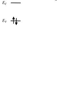
Fig. 2: Simplified model of the electronic structure of an InAs quantum box and of the filling of its states at thermal equilibrium at T = 0.
We consider that the energy levels in the conduction band, labeled by a positive integer n, are equally spaced and separated by ωc ; the energy of the fundamental level (n = 0) is noted Ec. The nth level is 2(n + 1) times degenerate, where the factor 2 accounts for the spin degeneracy and (n + 1) for the orbital degeneracy. Thus a conduction state is identified through the set of three in-
Problem 2001 : Quantum Boxes and Optoelectronics |
239 |
teger quantum numbers |n, l, s , with n > 0 and 0 ≤ l ≤ n, s = ±12 . The first
valence states are described in a similar way, with analogous notations (Ev ,ωv, n , l , s ).
I. Quantum Box in Thermal Equilibrium
At zero temperature and thermal equilibrium, the valence states are occupied by electrons, whereas the conduction states are empty. We are going to show in this section that the occupation factor of the conduction states of the quantum box in equilibrium remains small for temperatures up to 300K. Therefore, only in this part, the electronic structure of the quantum box will be roughly described by just considering the conduction and valence band levels lying nearest to the band gap. Fig.3 illustrates the assumed electronic configuration of the quantum box at zero temperature.
Fig. 3 : Electronic configuration at T = 0.
I.1. Give the average number of electrons in each of these two (spindegenerate) levels versus β = 1/kB T , where T is the temperature, and the chemical potential µ .
I.2. Find an implicit relation defining µ versus β, by expressing the conservation of the total number of electrons in the thermal excitation process.
I.3. Show that, in the framework of this model, µ is equal to (Ec + Ev )/2 independently of temperature.
I.4. Estimate the average number of electrons in the conduction level at 300K and conclude. For the numerical result one will take Ec − Ev = 1 eV.
In optoelectronic devices, like electroluminescent diodes or lasers, electrons are injected into the conduction band and holes into the valence band of the semiconducting active medium : the system is then out of equilibrium. The return toward equilibrium takes place through electron transitions from the conduction band toward the valence band, which may be associated with light emission.

240 |
Exercises and Problems |
Although the box is not in equilibrium, you will use results obtained in the course (for systems in equilibrium) to study the distribution of electrons in the conduction band, and that of holes in the valence band. Consider that, inside a given band, the carriers are in equilibrium among themselves, with a specific chemical potential for each band. This is justified by the fact that the phenomena responsible for transitions between conduction states, or between valence states, are much faster than the recombination of electronhole pairs.
One now assumes in sections II and III that the quantum box exactly contains one electron-hole pair (regime of weak excitation) : the total number of electrons contained in all the conduction states is thus equal to 1; the same assumption is valid for the total number of holes present in the valence states.
II. Statistical Study of the Occupation Factor of the Conduction Band States
II.1. Write the Fermi distribution for a given electronic state |n, l, s versus β = 1/kB T and µ, the chemical potential of the conduction electrons. Show that this distribution factor fn,l,s only depends of the index n ; it will be written fn in the following.
II.2. Expressing that the total number of electrons is 1, find a relation between µ and β.
II.3. Show that µ < Ec.
II.4. Show that fn is a decreasing function of n. Deduce that
1
fn ≤ (n + 1)(n + 2)
(Hint : give an upper bound and a lower bound for the population of electronic states of energy smaller or equal to that of level n).
II.5. Deduce that for states other than the fundamental one, it is very reasonable to approximate the Fermi-Dirac distribution function by a MaxwellBoltzmann distribution and this independently of temperature. Deduce that the chemical potential is defined by the following implicit relation :
1 |
= g(β, w) , with |
w = eβ(µ−Ec) |
|
|
|
2 |
|
|
|||
|
|
|
|
|
|
|
and |
g(β, w) = |
w |
+ w (n + 1)e−βn ωc |
(1) |
|
|
||||
|
w + 1 |
||||
|
|
|
|
n≥1 |
|

Problem 2001 : Quantum Boxes and Optoelectronics |
241 |
II.6. Show that the function g defined in II.5 is an increasing function of w and a decreasing function of β. Deduce that the system fugacity w decreases when the temperature increases and that µ is a decreasing function of T .
II.7. Specify the chemical potential limits at high and low temperatures.
II.8. Deduce that beyond a critical temperature Tc – to be estimated only in the next questions – it becomes legitimate to make a Maxwell-Boltzmann-type approximation for the occupation factor of the fundamental level.
II.9. Now one tries to estimate Tc. Show that expression (1) can also be written under the form :
1 |
= |
w |
− w + |
w |
(2) |
2 |
w + 1 |
(1 − e−β ωc )2 |
[Hint : as a preliminary, calculate the sum χ(β) = e−βn ωc and compare
n≥1
it to the sum entering into equation (1)].
II.10. Consider that the Maxwell-Boltzmann approximation is valid for the fundamental state if f0 ≤ e +1 1 . Hence deduce Tc versus ωc.
II.11. For a temperature higher than Tc show that :
fn = e−βn ωc |
(1 − e−β ωc )2 |
(3) |
2 |
|
|
III. Statistics of holes
III.1. Give the average number of electrons in a valence band state |n , l , s of energy En , versus the chemical potential µv of the valence electrons.
(Recall : µv is di erent from µ because the quantum box is out of equilibrium when an electron-hole pair is injected into it.)
III.2. Deduce the average number of holes hn ,l ,s present in this valence state of energy En . Show that the holes follow a Fermi-Dirac statistics, if one associates the energy −En to this fictitious particle. Write the hole chemical potential versus µv .
It will thus be possible to easily adapt the results of section II, obtained for the conduction electrons, to the statistical study of the holes in the valence band.
242 |
Exercises and Problems |
IV. Radiative lifetime of the confined carriers
Consider a quantum box containing an electron-hole pair at the instant t = 0 ; several physical phenomena can produce its return to equilibrium. In the present section IV we only consider the radiative recombination of the charge carriers through spontaneous emission : the deexcitation of the electron from the conduction band to the valence band generates the emission of a photon.
However an optical transition between a conduction state |n, l, s and a valence state |n , l , s is only allowed if specific selection rules are satisfied. For the InAs quantum boxes, one can consider, to a very good approximation, that for an allowed transition n = n , l = l and s = s and that each allowed optical transition has the same strength. Consequently, the probability per unit time of radiative recombination for the electron-hole pair is simply given by
1 |
= |
|
fn,l,s · hn,l,s |
(4) |
|
τ0 |
|||
τr |
|
|
||
|
|
n,l,s |
|
|
The time τr is called the radiative lifetime of the electron-hole pair; the time τ0 is a constant characteristic of the strength of the allowed optical transitions.
IV.1. Show that, if only radiative recombinations take place and if the box contains one electron-hole pair at t = 0, the average number of electrons in the conduction band can be written e r for t > 0.
nsec
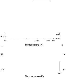
Fig. 4: Lifetime τ and radiative yield η measured for InAs quantum boxes; the curves are the result of the theoretical model developed in the present problem. The scales of τ, η and T are logarithmic.
IV.2. Now the temperature is zero. Calculate the radiative lifetime using (4).
The lifetime τ of the electron-hole pair can be measured. Its experimental variation versus T is shown in Fig. 4.
Problem 2001 : Quantum Boxes and Optoelectronics |
243 |
IV.3. Assume that at low temperature one can identify the lifetime τ and the radiative lifetime τr . Deduce τ0 from the data of Fig. 4.
IV.4. From general arguments show that the radiative lifetime τr is longer for T = 0 than for T = 0. (Do not try to calculate τr in this question.)
Now the temperature is in the 100–300K range. For InAs quantum boxes, some studies show that the energy spacing ω between quantum levels is of the order of 15 meV for the valence band and of 100 meV for the conduction band.
IV.5. Estimate Tc for the conduction electrons and the valence holes using the result of II.10. Show that a zero temperature approximation is valid at room temperature for the distribution function of the conduction states. What is the approximation then valid for the valence states?
IV.6. Deduce the dependence of the radiative lifetime versus temperature T for T > Tc.
IV.7. Compare to the experimental result for τ shown in Fig. 4. Which variation is explained by our model? What part of the variation remains unexplained?
IV.8. From the experimental values of τ at T = 200 K and at T = 0 K deduce an estimate of the energy spacing between hole levels. Compare to the value of 15 meV suggested in IV.4.
V. Non-Radiative Recombinations
trap
trap
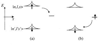
Fig. 5 : A simple two-step mechanism of non-radiative recombination.
The electron-hole pair can also recombine without emission of a photon (nonradiative recombination). A simple two-step mechanism of non-radiative recombination is schematized as follows : (a) a trap located in the neighborhood of the quantum box captures the electron; (b) the electron then recombines with

244 |
Exercises and Problems |
the hole, without emission of a photon. The symmetrical mechanism relying on the initial capture of a hole is also possible. One expects that such a phenomenon will be the more likely as the captured electron (or hole) lies in an excited state of the quantum box, because of its more extended wave function of larger amplitude at the trap location.
The radiative and non-radiative recombinations are mutually independent. Write 1/τnr for the probability per unit time of non-radiative recombination of the electron-hole pair; the total recombination probability per unit time is equal to 1/τ .
The dependence of the emission quantum yield η of the InAs quantum boxes is plotted versus T in the Fig. 4 above : η is defined as the fraction of recombinations occuring with emission of a photon.
V.1. Consider a quantum box containing an electron-hole pair at the instant t = 0. Write the di erential equation describing the evolution versus time of the average number of electrons in the conduction band, assuming that the electron-hole pair can recombine either with or without emission of radiation.
V.2. Deduce the expressions of τ and η versus τr and τnr .
V.3. Comment on the experimental dependence of η versus T . Why is it consistent with the experimental dependence of τ ?
Assume that the carriers, electrons or holes, can be trapped inside the nonradiative recombination center only if they lie in a level of the quantum box of large enough energy (index n higher than or equal to n0). Write the nonradiative recombination rate under the following form :
1
τnr
= γ (fn,l,s + tn,l,s) (5)
n≥n0 ,l,s
V.4. From the experimental results deduce an estimate of the index n0 for the InAs quantum boxes.
[Hint : work in a temperature range where the radiative recombination rate is negligible with respect to the non-radiative recombination rate and write a simple expression versus 1/T , to first order in η, then in ln η. You can assume, and justify the validity of this approximation, that the degeneracy of any level of index higher than or equal to n0 can be replaced by 2(n0 + 1)].
This simple description of the radiative and non-radiative recombination processes provides a very satisfactory understanding of the experimental dependences of the electron-hole pairs lifetime and of the radiative yield of the InAs
Problem 2002 : Physical Foundations of Spintronics |
245 |
quantum boxes (see Fig. 4). These experimental results and their modeling are taken from a study performed at the laboratory of Photonics and Nanostructures of the CNRS (French National Center of Scientific Research) at Bagneux, France.
Problem 2002 : Physical Foundations
of Spintronics
A promising research field in material physics consists in using the electron spin observable as a medium of information (spintronics). This observable has the advantage of not being directly a ected by the electrostatic fluctuations, contrarly to the space observables (position, momentum) of the electron. Thus, whereas in a standard semiconductor the momentum relaxation time of an electron does not exceed 10−12 sec, its spin relaxation time can reach 10−8 sec. Here we will limit ourselves to the two-dimensional motion of electrons (quantum well structure). The electron e ective mass is m. The accessible domain is the rectangle [0, Lx] × [0, Ly] of the xOy plane. The periodic limit conditions will be chosen at the edge of this rectangle. Part II can be treated if the results indicated in part I are assumed.
Part I : Quantum Mechanics
Consider the motion of an electron described by the hamiltonian
|
|
|
ˆ 2 |
|
|
|
ˆ |
= |
p |
+ α (ˆσxpˆx + σˆy pˆy ) |
α ≥ 0 |
|
H0 |
2m |
|||
ˆ |
|
|
|
|
|
where p |
= −i is the momentum operator of the electron and the σˆi (i = |
||||
x, y, z) represent the Pauli matrices. Do not try to justify this hamiltonian. Assume that at any time t the electron state is factorized into a space part
|
|
|
|
|
|
|
|
|
|
|
|
and a spin part, the space part being a plane wave of wave vector k. This |
|||||||||||
normalized state is thus written |
|
|
|
|
|
|
|
|
|||
|
|
|
|
|
|
|
a+(t) |
|
|||
|
eik·r |
|
|
|
eik·r |
|
|
|
|||
|
|
|
[a+(t)|+ + a−(t)|− ] = |
|
|
|
Åa−(t)ã |
(1) |
|||
|
|
|
|
|
|
||||||
|
|
LxLy |
|
LxLy |
|||||||
|
with|a+(t)| |
2 |
|
|
2 |
= 1 |
(2) |
||||
|
|
|
|
+ |a−(t)| |
|
|
|||||
where |± are the eigenvectors of σˆz . One will write kx = k cos φ, ky = k sin φ, with k ≥ 0, 0 ≤ φ < 2π.
246 |
Exercises and Problems |
I.1. Briefly justify that one can indeed search a solution of the Schroedinger equation under the form given in (2), where k and φ are time-independent. Write the evolution equations of the coe cients a±(t).
I.2 |
+(tã |
|
|
|
Åd |
|
|
(a) For fixed k and φ, show that the evolution of vector |
a+(t) |
des- |
|
a−(t) |
|||
|
|
a ) |
|
cribing the spin state can be put under the form : i |
|
Å a−(t) |
ã = |
dt |
|||
Åã
|
|
ˆ |
a+(t) |
|
|
|
ˆ |
|
× 2 hermitian matrix, that will be expli- |
||||||
|
Hs |
a−(t) |
|
where Hs is a 2 |
|||||||||||
|
citly written versus k, φ, and the constants α, and m. |
|
|
||||||||||||
(b) |
|
|
|
|
|
|
|
|
|
|
|
|
ˆ |
|
|
Show that the two eigenenergies of the spin hamiltonian Hs are : E± = |
|||||||||||||||
|
|
2k2 |
± α k with the corresponding eigenstates : |
|
|
|
|||||||||
|
|
2m |
|
|
|
||||||||||
|
|
|
|
1 |
1 |
|
|
1 |
|
1 |
|
|
|||
|
|
|
|χ+ = √ |
|
Å eiφ |
ã |
|χ− = √ |
|
Å −eiφ ã |
|
(3) |
||||
|
|
|
2 |
2 |
|
||||||||||
(c) |
Deduce that the set of |Ψk,± |
states : |
|
|
|
|
|
|
|||||||
|
|
|Ψk,+ = |
|
|
|
ã |
|Ψk,− = |
|
Å −eiφ |
ã |
(4) |
||||
|
|
|
2L·xLy Å eiφ |
2L·xLy |
|||||||||||
|
|
|
|
eik r |
1 |
|
|
eik r |
1 |
|
|
||||
|
with ki = 2πn |
i/Li |
(i = x, y and ni positive, negative or null integers) |
||||||||||||
|
constitute a basis, well adapted to the problem, of the space of the |
||||||||||||||
|
one-electron states. |
|
|
|
|
|
|
|
|
|
|||||
I.3 Assume that at t = 0 the state is of the type (2) and write ω = αk. |
|
||||||||||||||
(a) |
Decompose this initial state on the |Ψk,± basis. |
|
|
|
|||||||||||
(b) |
Deduce the expression of a±(t) versus a±(0). |
|
|
|
|
|
|
||||||||
I.4 One defines sz (t), the average value at time t of the z-component of the
ˆ
electron spin Sz = ( /2) σˆz . Show that :
sz (t) = sz (0) cos(2ωt) + sin(2ωt) Im a+(0) a−(0) e−iφ
I.5 The system is installed in a magnetic field B lying along the z-axis. The
|
|
|
|
|
|
|
|
|
e ect of B on the orbital variables is neglected. The hamiltonian thus becomes |
||||||||
ˆ ˆ |
ˆ |
|
|
|
|
|
|
|
H = H0 |
− γBSz . |
|
|
|
|
|
|
|
(a) Why does the momentum k remain a good quantum number? Deduce |
||||||||
|
|
|
|
|
|
ˆ (B) |
can still be defined. You |
|
that, for a fixed k, a spin hamiltonian Hs |
||||||||
|
ˆ |
|
|
|
|
|
|
|
will express it versus Hs, γ, B and σˆz . |
|
|
||||||
|
|
|
|
ˆ (B) |
are |
|
|
|
(b) Show that the eigenenergies of Hs |
|
|
||||||
|
(B) |
|
2k2 |
|
|
|
|
|
|
|
|
|
|
|
|||
|
E± |
= |
|
± »α2k2 + γ2B2/4 |
||||
|
2m |
|||||||
Problem 2002 : Physical Foundations of Spintronics |
247 |
|
|
|
|
|
|
|
|
|
|
|
|
|
|
|
|
|
|
|
|
|
|
|
|
(c) Consider a weak field B (γB αk). The expression of the eigenvectors |
|||||||||||||||||||||||
ˆ |
|
|
|
|
|
|
|
|
|
|
|
|
|
|
|
|
|
|
|
|
|
|
|
of Hs to first order in B are then given by |
|
|
|
|
|
|
|
|
|
|
|
|
|||||||||||
(B) |
= |
|
|
|
γB |
|
|
(B) |
= |χ− + |
|
γB |
|
|
|
|
||||||||
|χ+ |
|χ+ − |
|
|
|
|χ− |
|χ− |
|
|
|
|χ+ |
|
|
|||||||||||
|
4αk |
4αk |
|
|
|||||||||||||||||||
|
|
|
|
|
|
|
|
|
|
ˆ |
|
|
|
(B) |
are |
|
|
|
|
||||
Deduce that the average values of Sz in the states |χ± |
|
|
|
|
|||||||||||||||||||
(B) |
ˆ |
(B) |
|
= − |
γB |
(B) |
ˆ |
(B) |
= + |
γB |
|
|
|||||||||||
χ+ |
|
|Sz |χ+ |
|
|
|
χ− |
|
|Sz |χ− |
|
|
|
|
|||||||||||
|
4αk |
|
4αk |
|
|
||||||||||||||||||
|
|
|
|
|
|
(B) |
and of the matrix elements |
|
(B) |
ˆ |
(B) |
, |
|||||||||||
(d) What are the values of |χ± |
χ± |
|Sz |χ± |
|||||||||||||||||||||
in the case of a strong field B (such that γB αk).
Part II : Statistical Physics
In this part, we are dealing with the properties of an assembly of N electrons, assumed to be without any mutual interaction, each of them being submitted to the hamiltonian studied in Part I. We will first assume that there is no magnetic field; the energy levels are then distributed into two branches as obtained in I.2 :
E±(k) = |
2k2 |
|
|
(5) |
||
|
± α k |
|
|
|||
2m |
|
|
||||
|
= mα/ and 0 = |
2 |
2 |
2 |
||
with k = |k|. We will write k0 |
|
k0 |
/(2m) = mα /2. |
|||
II.1. We first consider the case α = 0. Briefly recall why the density of states D0( ) of either branch is independent of for this two-dimensional problem. Show that D0( ) = mLxLy/(2π 2).
II.2. We return to the real problem with α > 0 and now consider the branch
E+(k).
(a)Plot the dispersion law E+(k) versus k. What is the energy range accessible in this branch?
(b)Express k versus k0, 0, m, and the energy for this branch. Deduce the density of states :
|
|
|
|
D+( ) = D0( ) Å1 − … |
|
ã |
|
0 |
(6) |
||
+ 0 |
Plot D+( )/D0( ) versus / 0.
II.3. One is now interested by the branch E−(k).
(a)Plot E−(k) versus k and indicate the accessible energy range. How many k’s are possible for a given energy ?