

Statistical physics (2005)
.pdfxii |
Introduction |
of the field of Statistical Physics, which is not discussed in this book). Whether the system is in equilibrium or not, the parameters accessible to an experiment are just those of Thermodynamics. The purpose of Statistical Physics is to bridge the gap between the microscopic modeling of the system and the macroscopic physical parameters that characterize it (Ch. 2).
The studied system can be found in a great many states, solutions of the Quantum Mechanics problem, which di er by the values of their microscopic parameters while satisfying the same specified macroscopic physical conditions, for example a fixed number of particles and a given temperature. The aim is thus to propose statistical hypotheses on the likehood for a particular microscopic state or another one to be indeed realized in these conditions : the statistical description of systems in equilibrium is based on the postulate on the quantity statistical entropy : it should be maximum consistently with the constraints on the system under study. The treated problems concern all kinds of degrees of freedom : translation, rotation, magnetization, sites occupied by the particles, etc. For example, for a system made of N spins, of given total magnetization M , from combinatory arguments one will look for all the microscopic spin configurations leading to M ; then one will make the basic hypothesis that, in the absence of additional information, all the possible configurations are equally likely (Ch. 2). Obviously it will be necessary to verify the validity of the microscopic model, as this approach must be consistent with the laws and results of Thermodynamics (Ch. 3)
It is specified in the Quantum Mechanics courses that the limit of Classical Mechanics is justified when the de Broglie wavelength associated with the wavefunction is much shorter than all the characteristic dimensions of the problem. When dealing with free indistinguishable mobile particles, the characteristic length to be considered is the average distance between particles, which is thus compared to the de Broglie wavelength, or to the size of a typical wave packet, at the considered temperature.
According to this criterion, among the systems including a very large number of mobile particles, all described by Quantum Mechanics, two types will thus be distinguished, and this will lead to consequences on their Statistical Physics properties :
– in dilute enough systems the wave packets associated with two neighboring particles do not overlap. In such systems, the possible potential energy of a particle expresses an external field force (for example gravity) or its confinement in a finite volume. This system constitutes THE “ideal gas” : this means that all diluted systems of mobile particles, subjected to the same external potential, have the same properties, except for those related to the particle mass (Ch. 4);
Introduction |
xiii |
– in the opposite case of a high density of particles, like the atoms of a liquid or the electrons of a solid, the wave packets of neighboring particles do overlap. Quantum Mechanics analyzes this latter situation through the Pauli principle : you certainly learnt a special case of it, the Pauli exclusion principle, which applies to the filling of atomic levels by electrons in Chemistry. The general expression of the Pauli principle (Ch. 5) specifies the conditions on the symmetry of the wavefunction for N identical particles. There are only two possibilities and to each of them is associated a type of particle :
-on the one hand, the fermions, such that only a single fermion can be in a given quantum state;
-on the other hand, the bosons, which can be in unlimited number in a determined quantum state.
The consequences of the Pauli principle on the statistical treatment of noninteracting indistinguishable particles, i.e., the two types of Quantum Statistics, that of Fermi-Dirac and that of Bose-Einstein, are first presented in very general terms in Ch. 6.
In the second part of this course (Ch. 7 and the following chapters), examples of systems following Quantum Statistics are treated in detail. They are very important for the physics and technology of today. Some properties of fermions are presented using the example of electrons in metallic (Ch. 7) or, more generally, crystalline (Ch. 8) solids.
Massive boson particles, in conserved number, are studied using the examples of the superfluid helium and the Bose-Einstein condensation of atoms. Finally, the thermal radiation, an example of a system of bosons in non-conserved number, will introduce us into very practical current problems (Ch. 9).
A topic in physics can only be fully understood after su cient practice. A selection of exercises and problems with their solution is presented at the end of the book.
This introductory course of Statistical Physics emphasizes the microscopic interpretation of results obtained in the framework of Thermodynamics and illustrates its approach, as much as possible, through practical examples : thus the Quantum Statistics will provide an opportunity to understand what is an insulator, a metal, a semiconductor, or what is the principle of the greenhouse e ect that could deeply influence our life on earth (and particularly that of our descendants!).
The content of this book is influenced by the previous courses of Statistical Physics taught at Ecole Polytechnique : the one by Roger Balian From microphysics to macrophysics : methods and application to statistical physics, volume I translated by D. ter Haar and J.F. Gregg, volume II translated by D.
xiv |
Introduction |
ter Haar, Springer Verlag Berlin (1991), given during the 1980s; the course by Edouard Brézin during the 1990s. I thank them here for all that they brought to me in the stimulating field of Statistical Physics.
Several discussions in the present book are inspired from the course by F. Reif Fundamentals of Statistical and Thermal Physics, Mac Graw-Hill (1965), a not so recent work, but with a clear and practical approach, that should suit students attracted by the “physical” aspect of arguments. Many other Physical Statistics text books, of introductory or advanced level, are edited by Springer. This one o ers the point of view of a top French scientific Grande Ecole on the subject.
The present course is the result of a collective work of the Physics Department of Ecole Polytechnique. I thank the colleagues with whom I worked the past years, L. Auvray, G. Bastard, C. Bachas, B. Duplantier, A. Georges,
T.Jolicoeur, M. Mézard, D. Quéré, J-C. Tolédano, and particularly my coworkers from the course of Statistical Physics “A”, F. Albenque, I. Antoniadis,
U.Bockelmann, J.-M. Gérard, C. Kopper, J.-Y. Marzin, who brought their suggestions to this book and with whom it is a real pleasure to teach.
Finally, I would like to thank M. Digot, M. Maguer and D. Toustou, from the Printing O ce of Ecole Polytechnique, for their expert and good-humored help in the preparation of the book.
Glossary
We begin by recalling some definitions in Thermodynamics that will be very useful in the following. For convenience, we will also list the main definitions of Statistical Physics, introduced in the next chapters of this book. This section is much inspired by chapter 1, The Language of Thermodynamics, from the book Thermodynamique, by J.-P. Faroux and J. Renault (Dunod, 1997).
Some definitions of Thermodynamics :
The system is the object under study; it can be of microscopic or macroscopic size. It is distinguished from the rest of the Universe, called the surroundings.
A system is isolated if it does not exchange anything (in particular energy, particles) with its surroundings. The parameters (or state variables) are independent quantities which define the macroscopic state of the system : their nature can be mechanical (pressure, volume), electrical (charge, potential), thermal (temperature, entropy), etc. If these parameters take the same value at any point of the system, the system is homogeneous. The external parameters are independent parameters (volume, electrical or magnetic field) which can be controlled from the outside and imposed to the system, to the experimental accuracy. The internal parameters cannot be controlled and may fluctuate; this is the case for example of the local repartition of density under an external constraint. The internal parameters adjust themselves under the e ect of a modification of the external parameters.
A system is in equilibrium when all its internal variables remain constant in time and, in the case of a system which is not isolated, if it has no exchange with its surroundings : that is, there is no exchange of energy, of electric charges, of particles. In Thermodynamics it is assumed that any system, submitted to constant and uniform external conditions, evolves toward an equilibrium state that it can no longer spontaneously leave afterward. The thermal equilibrium between two systems is realized after exchanges between themselves : this is not possible if the walls which separate them are adiabatical, i.e., they do not transmit any energy.
xv
xvi |
Glossary |
In a homogeneous system, the intensive parameters, such as its temperature, pressure, the di erence in electrical potential, do not vary when the system volume increases. On the other hand, the extensive parameters such as the volume, the internal energy, the electrical charge are proportional to the volume.
Any evolution of the system from one state to another one is called a process or transformation. An infinitesimal process corresponds to an infinitely small variation of the external parameters between the initial state and the final state of the system. A reversible transformation takes place through a continuous set of equilibrium intermediate states, for both the system and the surroundings, i.e., all the parameters defining the system state vary continuously : it is then possible to vary these parameters in the reverse direction and return to the initial state. A transformation which does not obey this definition is said to be irreversible.
In a quasi-static transformation, at any time the system is in internal equilibrium and its internal parameters are continuously defined. Contrarly to a reversible process, this does not imply anything about the surroundings but only means that the process is slow enough with respect to the characteristic relaxation time of the system.
Some definitions of Statistical Physics :
A configuration defined by the data of the microscopic physical parameters, given by Quantum or Classical Mechanics, is a microstate.
A configuration defined by the data of the macroscopic physical parameters, given by Thermodynamics, is a macrostate.
An ensemble average is performed at a given time on an assembly of systems of the same type, prepared in the same macroscopic conditions.
In the microcanonical ensemble, each of these systems is isolated and its energy E is fixed, that is, it is lying in the range between E and E + δE. It contains a fixed number N of particles.
In the canonical ensemble, each system is in thermal contact with a large system, a heat reservoir, which imposes its temperature T ; the energy of each system is di erent but for macroscopic systems the average E is defined with very good accuracy. Each system contains N particles.
In the canonical ensemble the partition function is the quantity that norms the probabilities, which are Boltzmann factors. (see Ch. 2)
In the grand canonical ensemble, each system is in thermal contact with a heat
Glossary |
xvii |
reservoir which imposes its temperature T , the energy of each system being di erent. The energies of the various systems are spread around an average value, defined with high accuracy in the case of a macroscopic system. Each system is also in contact with a particle reservoir, which imposes its chemical potential : the number of particles di ers according to the system, the average value N is defined with high accuracy for a macroscopic system.
Chapter 1
Statistical Description of
Large Systems. Postulates
of Statistical Physics
The aim of Statistical Physics is to bridge the gap between the microscopic and macroscopic worlds. Its first step consists in stating hypotheses about the microscopic behavior of the particles of a macroscopic system, i.e., with characteristic dimensions very large with respect to atomic distances; the objective is then the prediction of macroscopic properties, which can be measured in experiments. The system under study may be a gas, a solid, etc., i.e., of physical or chemical or biological nature, and the measurements may deal with thermal, electrical, magnetic, chemical, properties. In the present chapter we first choose a microscopic description, either through Classical or Quantum Mechanics, of an individual particle and its degrees of freedom. The phase space is introduced, in which the time evolution of such a particle is described by a trajectory : in the quantum case, this trajectory is defined with a limited resolution because of the Heisenberg uncertainty principle (§1.1). Such a description is then generalized to the case of the very many particles in a macroscopic system : the complexity arising from the large number of particles will be suggested from the example of molecules in a gas (§1.2). For so large numbers, only a statistical description can be considered and §1.3 presents the basic postulate of Statistical Physics and the concept of statistical entropy, as introduced by Ludwig Boltzmann (1844-1906), an Austrian physicist, at the end of the 19th century.
1
2 |
Chapter 1. Statistical Description of Large Systems |
1.1Classical or Quantum Evolution of a Particle ; Phase Space
For a single particle we describe the time evolution first in a classical framework, then in a quantum description. In both cases, this evolution is conveniently described in the phase space.
1.1.1Classical Evolution
px 
t1
t0
O |
x |
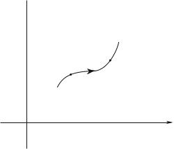
Fig. 1.1 : Trajectory of a particle in the phase space.
Consider a single classical particle, of momentum p0, located at the coordinate
r0 at time t0. It is submitted to a force F0(t). Its time evolution can be predicted through the Fundamental Principle of Dynamics, since
dp |
|
|
|
dt |
|
= F (t) |
(1.1) |
This evolution is deterministic since the set (r, p) can be deduced at any later time t. One introduces the one-particle “phase space”, at six dimensions, of coordinates (x, y, z, px, py, pz ). The data (r, p) correspond to a given point of this space, the time evolution of the particle defines a trajectory, schematized on the Fig. 1.1 in the case of a one-dimension space motion. In the particular case of a periodic motion, this trajectory is closed since after a period the particle returns at the same position with the same momentum : for example the abscissa x and momentum px of a one-dimension harmonic oscillator of
Classical or Quantum Evolution of a Particle |
3 |
mass m and frequency ω are linked by :
px2 |
1 2 2 |
|
||
|
+ |
|
mω x = E |
(1.2) |
2m |
2 |
|||
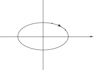
In the phase space this relation is the equation of an ellipse, a closed trajectory periodically described (Fig. 1.2). Another way of determining the time
px
t0
t1
O |
E |
x |
Fig. 1.2: Trajectory in the phase space for a one-dimension harmonic oscillator of energy E.
evolution of a particle is to use the Hamilton equations (see for example the course of Quantum Mechanics by J.-L. Basdevant and J. Dalibard, including a CDROM, Springer, 2002) : the motion is deduced from the position r and its corresponding momentum p. The hamiltonian function associated with the total energy of the particle of mass m is given by :
|
p2 |
|
|
h = |
|
+ V (r) |
(1.3) |
|
|||
|
2m |
|
|
where the first term is the particle kinetic energy and V is its potential energy, from which the force in (1.1) is derived. The Hamilton equations of motion are given by :
|
|
|
∂h |
|
||||
|
|
|
|
|
|
|
|
|
|
˙ |
|
∂h |
|
||||
|
p = − |
|
∂r |
(1.4) |
||||
|
|
r˙ = ∂p |
||||||
|
Fundamental |
|
|
|
|
|||
and are equivalent to the |
Relation of Dynamics (1.1). |
|
||||||
|
|
|
|
|
|
|
|
|
Note : Statistical Physics also applies to relativistic particles which have a di erent energy expression.
4 |
Chapter 1. Statistical Description of Large Systems |
1.1.2Quantum Evolution
It is well known that the correct description of a particle and of its evolution requires Quantum Mechanics and that to the classical hamiltonian function h
ˆ
corresponds the quantum hamiltonian operator h. The Schroedinger equation provides the time evolution of the state |ψ :
|
∂t |
|
| |
|
|
i |
∂|ψ |
= hˆ |
ψ |
|
(1.5) |
|
|
The squared modulus of the spatial wave function associated with |ψ gives the probability of the location of the particle at any position and any time. Both in Classical and Quantum Mechanics, it is possible to reverse the time direction, i.e., to replace t by −t in the motion equations (1.1), (1.4) or (1.5), and thus obtain an equally acceptable solution.
1.1.3Uncertainty Principle and Phase Space
You know that Quantum Mechanics introduces a probabilistic character, even when the particle is in a well-defined state : if the particle is not in an ei-
ˆ
genstate of the measured observable A, the measurement result is uncertain. Indeed, for a single measurement the result is any of the eigenvalues aα of the considered observable. On the other hand, when this measurement is reproduced a large number of times on identical, similarly prepared systems, the
| ˆ|
average of the results is ψ A ψ , a well-defined value.
px |
|
|
h |
O |
x |
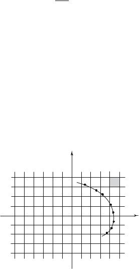
Fig. 1.3: A phase space cell, of area h for a one-dimension motion, corresponds to one quantum state.