Scales: This option draws numeric scales along each axis.
Background: This option paints the three coordinate planes clear when disabled, regardless of their color settings.
Flash Cursor: This option flashes the two numeric cursors for easier visibility.
Patches:
X: This controls the number of patches along the X axis. This number defaults to 40. It may be as high as you wish, but remember, the number of total patches is equal to the product of the number of X and Z patches. Picking 40 for each axis requires 40*40 = 1600 patches. Picking 1000 for each axis requires 1000*1000 = 1,000,000 patches. Each patch must be imaged through a set of 3D trigonometric transforms. These take time to calculate and slow down the drawing. Also, with more than 200 patches the surface is covered with isolines lines spaced so close it's hard to see the surface, so limit this value to 20 to 200.
Z: This controls the number of patches along the Z axis. The same considerations as for the X axis apply here as well.
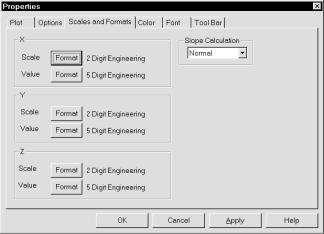
Scales and Formats: This panel accesses the numeric format features of the 3D graph. Its options are shown below:
Figure 27-8 The Format panel of the 3D dialog box
For each of the three axes, X, Y, and Z, you can control the Scale and Value numeric format.
Scale Format: This is the numeric format used to print the X axis scale. There are two basic formats:
Value Format: This numeric format is used to print the curve's X, Y, and Z values in the table below the plot in Cursor mode. Its format is the same as the scale format described above.
• Slope Calculation: This lets you select among three forms of slope calculation: Normal, dB/Octave, and dB/Decade.
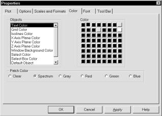
Color:This panel accesses the color features. The panel looks like this:
Figure 27-9 The Color panel of the 3D dialog box
This panel lets you control the color of the following features:
Objects: This group includes the color of the grid, text, isolines, X, Y, and Z axis planes, and the window background. To change an object's color, first select it, then select a new color from the palette.
Patch Color: This panel lets you control the color of the patches that comprise the 3D surface. You can choose from:
•Clear: This option leaves the patches transparent, producing what looks like a wire mesh if the Isolines option is enabled, or no plot at all if it isn't enabled.
•Spectrum: This option colors the patches with the colors of the spectrum ranging from blue for the lowest values to red for the largest values.
•Gray: This option colors the patches with shades of gray that range from black for the low values to white for the high values.
•Red: This option colors the patches with shades of red that range from dark red for the low values to light red for the high values.
•Green: This option colors the patches with shades of green that range from dark green for the low values to light green for the high values.
•Blue: This option colors the patches with shades of blue that range from dark blue for the low values to light blue for the high values.
• Font
This standard panel lets you select font, style, size, and effects for all of the text used in the 3D plot.
• Tool Bar
This standard panel lets you select the buttons that will appear in the local tool bar of the 3D window.
To add a 3D plot window, select Transient / 3D Windows / Add 3D Window. This displays a new 3D Properties dialog box and lets you select the desired plot features.
Cursor mode in 3D
As with normal 2D plots, a Cursor mode is available to numerically examine the
3D plot. Press F8 or click on the Cursor mode  button. The 3D plot will now look like this:
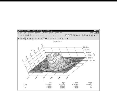
Figure 27-11 The 3D plot in Cursor mode
Click the mouse somewhere near the middle of the 3D surface plot. A cursor should appear. Press the LEFT ARROW key several times. Press the RIGHT ARROW key several times. Notice that the cursor selects a changing set of X axis, or T, values, but moves along a grid of constant Z axis, or R(R1), value.
Press the DOWN ARROW key several times. Press the UP ARROW key several times. Notice that the cursor selects a changing set of Z axis, or R(R1), values, but moves along a grid of constant X axis, or T, value.
All of the usual Cursor function modes are available. In particular the Next, Peak, Valley, High, Low, Inflection, Global High, Global Low, Go To X, Go To Y, and Go To Performance modes are available. For example, click on the Peak button. Press the RIGHT ARROW cursor key several times. The left numeric cursor is placed on each successive peak of the constant Z, or R(R1), curve.
3D Performance functions
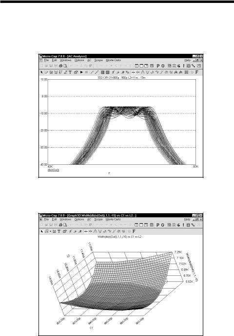
To illustrate how to select performance functions for 3D plotting, load the file 3D2. Select AC from the Analysis menu. Press F2 to start the runs. The runs looklikethis:
Figure 27-12 The 3D2 runs
Select AC / 3D Windows / Width... This produces the following plot:
Figure 27-13 The plot of Width vs. L2 and C1
Here we have plotted the Width performance function:
Width(db(v(Out)),1,1,-15)
This performance function measures the width of the db(V(Out)) function at a Boolean of 1 (always true), first instance, at the Y value of -15. This effectively measures the -15 db bandwidth of the bandpass filter.
The value of L2 is stepped from 11mh to 13mh, in steps of .25mh, while stepping C1 from 800pf to 900pf in steps of 25pf. This produces 9*5, or 45 runs. The width is measured for each of these runs and the 3D graph plots the value of the Width function vs. the C1 value along the X axis and the L2 value along the Z axis. The plot shows how the filter bandwidth varies with C1 and L2.
Select AC / 3D Windows / Y_Range(). This produces the following plot:
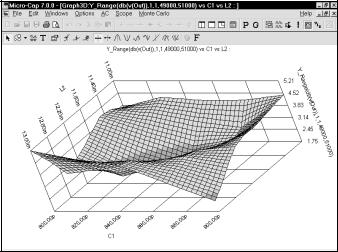
Figure 27-14 The plot of Y_Range vs. L1 and C2
Here we've plotted the Y_Range performance function:
Y_Range(db(v(Out)),1,1,49000,51000)
This performance function measures the variation of the db(V(Out)) function at a Boolean of 1 (always true), first instance, over the X range of 49Khz to 51Khz. This effectively measures the passband ripple of the filter.
Changing the plot orientation
The orientation of the 3D plot can be changed in several ways:
•By dragging the axis endpoints with the mouse.
•By using the keyboard
•Q: Rotates the plot clockwise about the X axis.
•A: Rotates the plot counter clockwise about the X axis.
•W: Rotates the plot clockwise about the Y axis.
•S: Rotates the plot counter clockwise about the Y axis.
•E: Rotates the plot clockwise about the Z axis.
•D: Rotates the plot counter clockwise about the Z axis.
•X: View from perpendicular to the X=0 plane.
•Y: View from perpendicular to the Y=0 plane.
•Z: View from perpendicular to the Z=0 plane.
•CTRL + HOME: Standard view orientation.
•C: Toggles between contour and 3D view.
Scaling in 3D
The choice of scaling is determined entirely by the range of axis variables. There is no user control of scaling.
What's in this chapter
The optimizer included with MC7 uses a variation of the Powell direction-set method for optimization. It is a robust technique that works well for the kinds of optimization problems found in circuit design.
The chapter is organized as follows:
How the optimizer works
The Optimize dialog box
Optimizing low frequency gain
Optimizing matching networks
Curve fitting with the optimizer
How the optimizer works
The optimizer systematically changes user-specified parameters to maximize, minimize, or equate a chosen performance function, while keeping the parameters within prescribed limits and conforming to any specified constraints.
It works in any analysis mode, letting you optimize transient, AC small-signal or DC characteristics. Anything that can be measured in any analysis mode by any performance function can be maximized, minimized, or equated. Equating is the process of matching specified points on a curve. A typical application would be trying to match points on a Bode plot gain curve.
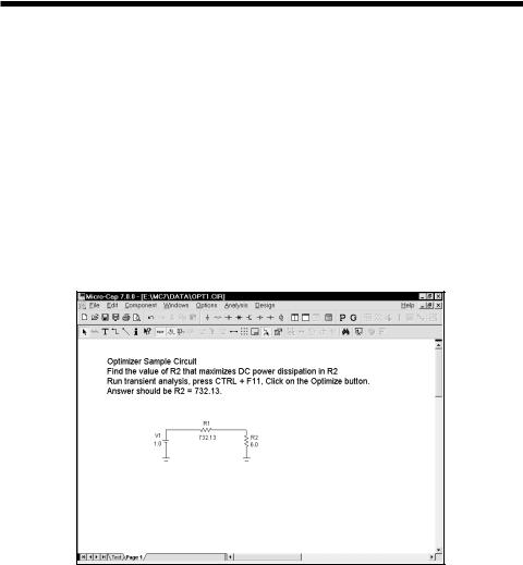
To see how optimization works, load the file circuit OPT1.CIR. It looks like this:
Figure 28-1 The OPT1 circuit
This circuit delivers power to a 6.0 ohm load from a 1.0 volt battery through a 732.13 ohm source resistance. We'll use the optimizer to find the value of R2 that maximizes its power.
656 Chapter 28: Optimizer