Micro-Cap v7.1.6 / RM

Transmission line

SPICE format

Ideal Line

T<name> <A port + node> <A port - node> +<B port + node> <B port - node> +[model name]

+ Z0=<value> [TD=<value>] | [F=<value> [NL=<value>]]

Example

T1 10 20 30 40 Z0=50 TD=3.5ns

T1 10 20 30 40 Z0=150 F=125Meg NL=0.5

T1 20 30 40 50 TLMODEL

Lossy Line

T<name> <A port + node> <A port - node> +<B port + node> <B port - node> +[<model name> [physical length]]

+LEN=<len value> R=<rvalue> L=<lvalue> G=<gvalue>

+C=<cvalue>

Examples

T1 20 30 40 50 LEN=1 R=.5 L=.8U C=56PF

T3 1 2 3 4 TMODEL 12.0

Schematic format

PART attribute <name>

Example

T1

VALUE attribute for ideal line

Z0=<value> [TD=<value>] | [F=<value> [NL=<value>]]

Example for ideal line

Z0=50 TD=3.5ns

VALUE attribute for lossy line

<physical length> LEN=<len value> R=<rvalue> L=<lvalue> G=<gvalue> C=<cvalue>

478 Chapter 22: Analog Devices

Examples for lossy line

LEN=1 R=.5 L=.8U C=56PF

R=.5 L=.8U C=56PF

MODEL attribute <model name>

Example

RELAY

Model statement form

.MODEL <model name> TRN ([model parameters])

Examples

.MODEL TIDEAL TRN(Z0=50 TD=10ns)

.MODEL TLOSS TRN(C=23pf L=13nh R=.35)

LEN, R, L, G, and C must use a common unit of length. For example, if C is measured in units of farads/cm, then R must be in ohms/cm, L must be in henrys/cm, G must be in mhos/cm, and LEN must be in centimeters.

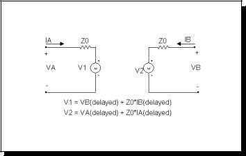
Model Equations

The ideal and lossy lines are represented by the model shown in Figure 22-20. The principal difference between the two models is in the implementation of the delay. In the ideal model, the delay is implemented as a linked-list of data pairs (time,value) and breakpoints.

479

User file source

Schematic format

PART attribute <name>

Example

U1

FILE attribute <file name>

Example

AMP.USR

EXPRESSION attribute [expression]

Example

V(10)+V(11)

The User file source is a voltage source whose waveform or curve comes from an ASCII text file. The files contain a header and N sequential lines, each with a variable number of data values:

AC:

Three data values per line: Frequency, Real(Y), Imag(Y) X set to Frequency Five data values per line: Frequency, Real(X), Imag(X), Real(Y), Imag(Y)

DC: Three data values per line:

DCINPUT1, X, Y

where X is the X expression value, Y is the Y expression value, and DCINPUT1 is the value of variable1.

User files may be created using a text editor, by external software, or by saving one or more curves or waveforms after an analysis run. To save a particular

481

waveform, press F10 to invoke the Plot Properties dialog box after the analysis is over and select the waveform to be saved from the Save Curves section of the dialogbox.

When you place a user source in a schematic, MC7 reads the current data directory to find any files with the extension *.USR. It then reads the files themselves to see what waveforms are available for use. It presents the files and waveforms as items in drop-down lists in the FILE and EXPRESSION fields so you can easily select the file name and waveform expression.

Curves saved in user files can be displayed directly in an analysis simply by selecting them from the Curves section of the Variables list. To invoke the Variables list, click in the Y Expression field and click the right mouse button. The X and Y parts of a waveform are stored as CurveX and CurveY, to let you select the X and Y parts independently.

See the files USER and USER2 for examples of how to use this type of source. Here is the SAMPLE.USR user file as an example of the format used:

[Main]

FileType=USR

Version=2.00 Program=Micro-Cap [Menu]

;Simple = T,X,Y

;SimpleNoX = T,Y ;Complex = F,Xr,Xi,Yr,Yi ;ComplexNoX=F,Yr,Yi

;FormatType = Simple | Complex | SimpleNoX | ComplexNoX ;Format=FormatType

WaveformMenu=label vs T [Waveform]

Label=label vs T MainX=T LabelX=T LabelY=label vs T Format=Simple

Data Point Count=256 0,0,0

2.352941176E-009,2.352941176E-009,0

4.705882353E-009,4.705882353E-009,0

...

482 Chapter 22: Analog Devices

W (Current-controlled switch)

SPICE format

W<name> <plus output node> <minus output node> +<controlling voltage source name> <model name>

Example

W1 10 20 V1 IREF

Schematic format

PART attribute <name>

Example

W1

REF attribute

<controlling voltage source name>

Example

VSENSE

MODEL attribute <model name>

Example

SW

This two terminal device, current-controlled switch is controlled by the current through the source defined by <controlling voltage source name>. The model parameters RON and ROFF must be greater than zero and less than 1/Gmin.

Do not make the ratio ROFF/RON larger than about 15 decades. The 15 digits of precision used by the simulator can not make meaningful use of a spread greater than 15 in the ratio. Do not make the transition region, ION-IOFF, too small as this will cause an excessive number of time points required to cross the region. The smallest value for ION-IOFF is (RELTOL•(max(ION,IOFF))+ABSTOL).

Model statement form

.MODEL <model name> ISWITCH ([model parameters])

483

Example

.MODEL W1 ISWITCH (RON=1 ROFF=1K ION=1 IOFF=1.5)

If ION > IOFF

If IC >= ION

RS = RON

If IC <= IOFF

RS = ROFF

If IOFF < IC < ION

RS = exp(LM + 3•LR•(IC-IM)/(2•ID) - 2•LR•(IC-IM)3/ID3)

If ION < IOFF

If IC <= ION

RS = RON

If IC >= IOFF

RS = ROFF

If IOFF > IC > ION

RS = exp(LM - 3•LR•(IC-IM)/(2•ID) + 2•LR•(IC-IM)3/ID3)

Noise effects

Noise is modeled as a resistor equal to the resistance found during the DC operating point. The thermal noise current is calculated as follows:

I= sqrt(4•k•T/RS)

484 Chapter 22: Analog Devices

486 Chapter 22: Analog Devices