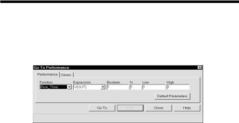
The Performance Function dialog box
These functions may be used on a single analysis plot, in Monte Carlo analysis, and in 3D plotting. When a run is complete, click on the Go To Performance
Function button. The dialog box looks like this:
Figure 26-1 Performance Function dialog box
There are two panels: Performance and Cases. The Cases panel lets you select a branch if more than one is available due to stepping. The Performance panel lets you select a performance function to apply to the selected curve branch chosen from the Cases panel.
The Performance panel provides the following fields:
Function: This selects one of the Performance functions.
Expression: This selects the expression for the function to work on. Only expressions that were plotted during the run are available.
Boolean: This Boolean expression must be true for the performance functions to consider a data point for inclusion in the search. Typically this function is used to exclude some unwanted part of the curve from the function search. A typical expression here would be "T>100ns". This would instruct the program to exclude any data points for which T<=100ns.
N: This integer specifies which of the instances you want to find and measure. For example, there might be many pulse widths to measure. Number one is the first one on the left starting at the first time point. The value of N is incremented each time you click on the Go To button, measuring each succeeding instance.
Low: This field specifies the low value to be used by the search routines. For example, in the Rise_Time function, this specifies the low value at which the rising edge is measured.
High: This field specifies the high value to be used by the search routines. For example, in the Rise_Time function, this specifies the high value at which the rising edge is measured.
Level: This field specifies the level value to be used by the search routines. For example, in the Width function, this specifies the expression value at which the width is measured.
The buttons at the bottom provide these functions:
Go To (Left): This button is called Go To when the performance function naturally positions both cursors (as the Rise_Time and Fall_Time functions do). It is named Left when either the left or right cursor, but not both, would be positioned by the function. When named Left, this button places the left numeric cursor at the position dictated by the performance function.
Right: This button places the right numeric cursor at the position dictated by the performance function. For example, the Peak function can position either the left or right cursor.
Close: This button closes the dialog box.
Default Parameters: This button calculates default parameters for functions which have them. It guesses at a suitable value by calculating the average value or the 20% and 80% points of a range.
Performance functions all share certain basic characteristics:
A performance function at its core is a search: The set of data points of the target expression is searched for the criteria specified by the performance function and its parameters.
Performance functions find the N'th instance: Every performance function has a parameter N which specifies which instance of the function to return. The only exceptions are the High and Low functions for which, by definition, there is a maximum of one instance.
628 Chapter 26 Performance Functions
Each performance function call increments the N parameter: Every time a performance function is called, N is incremented after the function is called. The next call automatically finds the next instance, and moves the cursor(s) to subsequent instances. For example, each call to the Peak function locates a new peak to the right of the old peak. When the end of the curve is reached, the function rolls over to the beginning of the curve.
Only curves plotted during the run can be used: Performance functions operate on curve data sets after the run, so only curves saved (plotted) during the run are available for analysis.
Boolean expression must be TRUE: Candidate data points are included only if the Boolean expression is true for the data point. The Boolean expression is provided to let the user include only the desired parts of the curve in the performance function search.
At least PERFORM_M neighboring points must qualify: If a data point is selected, the neighboring data points must be consistent with the search criteria or the point is rejected. For example, in the peak function, a data point is considered a peak if at least PERFORM_M data points on each side have a lower Y expression value. PERFORM_M is a Global Settings value and defaults to 1. Use 2 or even 3 if the curve is particularly choppy or has any trapezoidal ringing in it.
Performance function plots
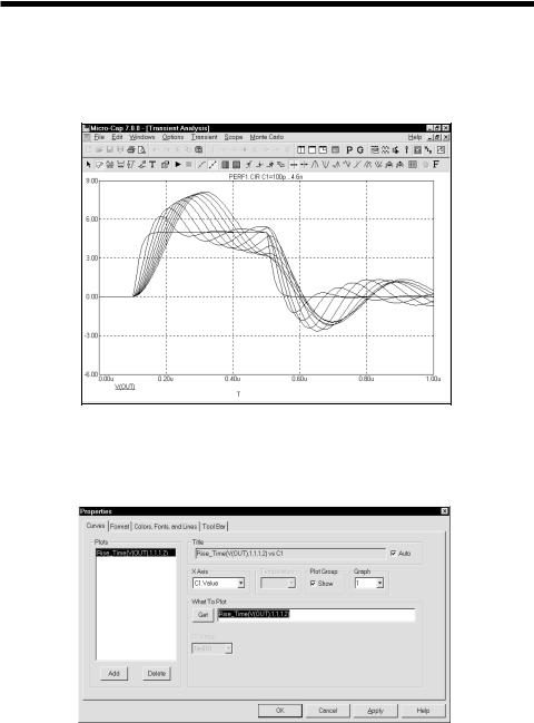
Performance Function plots may be created when multiple analysis runs have been done with temperature or parameter stepping. To illustrate, load the file PERF1. Run transient analysis. The plot should look like this:
Figure 26-2 The transient analysis run
From the Transient menu, select Performance Windows - Add Performance Window. This presents the Properties dialog box for performance plots.
Figure 26-3 The Properties dialog box for performance plots
630 Chapter 26 Performance Functions
The Plot Properties dialog box lets you control the performance plot window. It can be used for controlling the performance plot display after or even before the plot. The dialog box provides the following choices:
• Plot
Curves: This list box lets you select the curve that the performance functions will operate on. The Add and Delete buttons at the bottom let you add or delete a particular performance plot.
Title: This field lets you specify what the plot title is to be. If the Auto button is checked, the title is automatically created from the circuit name and analysis run details.
X Axis: This lets you select the stepped variable to use for the X axis.
Temperature: If temperature was also stepped, each value creates a separate curve. This lets you select the temperature whose curve the performance functions will operate on.
Curve: This check box controls whether the selected performance curve will be plotted or not. If you want to hide the curve from the plot group, remove the check mark by clicking in the box.
Plot Group: This group's list box controls the plot group number.
What To Plot: This group lets you select the performance function and its parameters.
Stepped Variables List: If more than one variable has been stepped, there will be one or more List boxes. These list boxes let you select which instance of the stepped variable(s) the performance functions
will process. For instance, if you stepped R1, L1, and C1 through 5 values each and chose R1 for the x axis variable, there would be a list box for L1 and one for C1. From these two lists, you could select any of the
5 X 5 = 25 possible curves and plot a performance function versus the R1 value.
• Format
Curves: This list box lets you select the plot that the other fields apply to.
X:This group includes:
Range Low: This is the low value of the X range used to plot the selected curve.
Range High: This is the high value of the X range used to plot the selected curve.
Grid Spacing: This is the distance between X grids.
Bold Grid Spacing: This is the distance between bold X grids.
Scale Format: This accesses a dialog box where you select the numeric format used to print the X axis scale.
Value Format: This accesses a dialog box where you select the numeric format used to print the curve's X value in the table below the plot in Cursor mode and in the tracker boxes.
Auto Scale: This command scales the X Range and places the numbers into the Low, High, and Grid Spacing fields. The effect on the plot can be seen by clicking the Apply button.
Log: If checked this makes the scale log.
Y: This group provides a similar set of commands for the Y axis group.
Same Y Scales: Enabling this check box forces the Auto Scale command to use a single common scale for all plots within a plot group. If the box is unchecked, the Auto Scale function will generate multiple scales for each plot in a plot group.
Use Common Formats: Clicking this button copies the X and Y formats of the selected curve to format fields of all plots.
• Colors, Fonts, and Lines
Objects: This list box lets you select the object that the other commands (color, font, lines) apply to. These include:
General Text: This is text used for axis scales, titles, cursor tables, and curve name.
632 Chapter 26 Performance Functions
Grid: This is the analysis plot grid.
Graph Background: This is the analysis plot background.
Window Background: This is the window background.
Select: This is the Select mode.
Select Box: This is the Select mode box.
Initial Object: This governs the initial properties of analysis text, graphical objects, and numeric tags added to the plot. Object properties can be changed after they are added to a plot by double-clickingonthem.
Tracker: These are the trackers.
Plot Names: These are the curve names.
Varied (Color): This group whose name changes to reflect the selected object, lets you change its color.
Curve Line: This group lets you change the color, width, and pattern of the plot object. The Rainbow option is not available. Windows 95 and 98 have pattern control only if the width is equal to 1. NT systems provide pattern control for any width.
Font: This group lets you change the font of the selected object.
Size: This group lets you change the text size of the selected object.
Style: This group lets you change the text style of the selected object.
Effects: This group lets you change text effects of the selected object.
Sample: This group shows a sample object using the currently selected font, color, width, and pattern properties appropriate to the object.
• Tool Bar:
This page lets you select the buttons that will appear in the local tool bar area below the Main tool bar.
Tool Bar: This list box lets you select the different local tool bars.
Buttons: This box lets you select the buttons that are to appear in the selected tool bar.
Show Button: If checked, the selected button is shown in the selected tool bar.
Top: If enabled, the tool bar is placed at the top part of the window.
Left: If enabled, the tool bar is placed at the left part of the window.
All On: This command places all buttons in the tool bar.
All Off: This command places no buttons in the tool bar.
Default: This command places the default set of buttons in the tool bar.
The four buttons at the bottom have the following functions:
OK: This button accepts all changes, exits the dialog box, and redraws the performance plot. Subsequent runs will use the changed properties and they will be retained in the circuit file, if the file itself is later saved.
Cancel: This button rejects all changes, exits the dialog box, and redraws the analysis plot using the original properties.
Apply: This button displays the analysis plot using the current settings in the dialog box to show how the display would be affected by the changes. The changes are still tentative, until the OK button is clicked.
Help: This button accesses local help information.
634 Chapter 26 Performance Functions
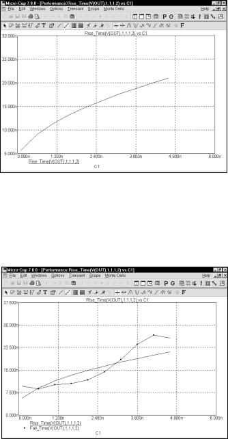
Click on the OK button. This selects the Rise_Time function with default parameters and creates the following performance plot.
Figure 26-4 Rise time performance plot
This plots shows how the rise time of V(1) (as measured between 1 and 2 volts) varies with the value of C1, the only stepped variable. Double-click on the graph or press F10. This invokes the Properties dialog box. Click on the Add button. Click on the Get button and select Fall_Time from the Function list box. This adds the Fall_Time function plot to the performance window. It looks like this:
Figure 26-5 Rise and fall time performance plots
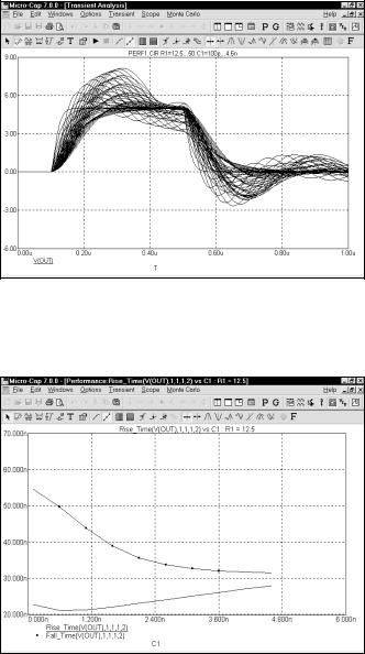
The window shows plots of both the Rise_Time and Fall_Time functions. Press F11 and click the Yes item in the Step It group of the Parameter 2 panel. Hit OK and press F2. The runs look like this:
Figure 26-6 Stepping both C1 and R1
Press CTRL + F6 until you see the performance plot. It should look like this:
Figure 26-7 Performance plots for R=12.5
636 Chapter 26 Performance Functions