7.2 Origin and Consequences of Magnetic Order |
397 |
|
|
where Rj is defined by (2.171) and cyclic boundary conditions are used so that the k are defined by (2.175). N = N1N2N3 and so the delta function relations (2.178) to (2.184) are valid. k will be assumed to be restricted to the first Brillouin zone. Using all these results, we can derive the inverse transformation
a j |
= |
1 |
∑k exp(−ik R j )Bk , |
(7.180a) |
|
|
N |
|
|
and |
|
|
|
|
a†j |
= |
1 |
∑k exp(ik R j )Bk† . |
(7.180b) |
|
|
N |
|
|
So far we have not shown that the B are boson creation and annihilation operators. To show this, we merely need to show that the B satisfy the appropriate commutation relations. The calculation is straightforward, and is left as a problem to show that the Bk obey the same commutation relations as the aj.
We can give a very precise definition to the word magnon. First let us review some physical principles. Exchange coupled spin systems (e.g. ferromagnets and antiferromagnets) have low-energy states that are wave-like. These wave-like energy states are called spin waves. A spin wave is quantized into units called magnons. We may have spin waves in any structure that is magnetically ordered. Since in the low-temperature region there are only a few spin waves that are excited and thus their complicated interactions are not so important, this is the best temperature region to examine spin waves. Mathematically, precisely whatever is created by Bk† and annihilated by Bk is called a magnon.
There is a nice theorem about the number of magnons. The total number of magnons equals the total spin deviation quantum number. This theorem is easily proved as shown below:
S= ∑ j (S − S jz ) = ∑ j a†a j
=N1 ∑i,k,k′exp[i(k − k′) R j ]Bk†Bk′
=∑k,k′δkk′Bk†Bk′
=∑k Bk†Bk .
This proves the theorem, since Bk†Bk is the occupation number operator for the number of magnons in mode k.
The Hamiltonian defined by (7.178) will now be approximated. The spin-wave variables Bk will also be substituted.
At low temperatures we may expect the spin-deviation quantum number to be rather small. Thus we have approximately
398 7 Magnetism, Magnons, and Magnetic Resonance
This implies that the relation between the S and a can be approximated by
− |
|
|
† |
|
† † |
|
|
|
|
|
− |
a j a j a j |
, |
(7.182a) |
S j |
2S a j |
4S |
|
|
|
|
|
|
|
|
|
|
|
|
|
|
|
|
|
|
+ |
|
|
|
|
† |
|
|
|
|
|
|
− |
a j a j a j |
, |
(7.182b) |
S j |
2S a j |
4S |
|
|
|
|
|
|
|
|
|
|
|
|
|
|
|
|
|
|
and
S jz = S − a†j a j .
Expressing these results in terms of the B, we find
S +j |
|
2S |
{∑k exp(−ik R j )Bk |
|
|
|
|
|
|
N |
|
|
|
|
|
}, |
|
− |
1 |
∑ |
k,k′,k′′ |
exp[i(k − k′ |
− k′′) R j ] B†B |
B |
|
4SN |
|
|
|
|
|
k k′ |
k′′ |
|
S −j |
|
2S |
{∑k exp(ik R j )Bk |
|
|
|
|
|
|
N |
|
|
|
|
|
}, |
|
− |
|
1 |
∑ |
k,k′,k′′ |
exp[i(k + k′ |
− k′′) R j ] B†B† |
B |
|
|
4SN |
|
|
|
|
|
k k′ |
k′′ |
|
and
S jz = S − N1 ∑k,k′exp[i(k − k′) R j ] Bk†Bk′ .
(7.182c)
(7.183a)
(7.183b)
(7.183c)
The details of the calculation begin to get rather long at about this stage. The approximate Hamiltonian in terms of spin-wave variables is obtained by substituting (7.183) into (7.178). Considerable simplification results from the delta function relations. Terms of order ( ai†ai /S)2 are to be neglected for consistency. The final result is
neglecting a constant term, where Z is the number of nearest neighbors, H0 is the term that is bilinear in the spin wave variables and is given by
|
H 0 = −JSZ[∑k (αk (1+ Bk†Bk ) +α−k Bk†Bk − 2Bk†Bk )] |
(7.185) |
|
+ gμB (μ0H )∑k Bk†Bk , |
|
|
|
α |
k |
= |
1 |
∑ exp(ik ) , |
(7.186) |
|
|
|
|
|
Z |
|
7.2 Origin and Consequences of Magnetic Order |
399 |
|
|
and Hex is called the exchange interaction Hamiltonian and is biquadratic in the spin-wave variables. It is given by
|
H ex Z |
J |
∑k k |
k |
k |
|
δkk2++kk3 (Bk |
|
Bk† |
−δkk2 )Bk† |
Bk |
|
(αk |
−αk |
−k |
) . (7.187) |
|
N |
4 |
1 |
4 |
|
|
1 |
2 |
3 |
|
1 |
4 |
2 |
1 |
3 |
|
1 |
1 |
|
2 |
Note that H0 describes magnons without interactions and Hex includes terms that describe the effect of interactions. Mathematically, we do not want to consider interactions. Physically, it makes sense to believe that interactions should not be important at low temperatures. We can show that Hex can be neglected for longwavelength magnons, which should be the only important magnons at low temperature. We will therefore neglect Hex in all discussions below.
H0 can be somewhat simplified. Incidentally, the formalism that is being used assumes only one atom per unit cell and that all atoms are equally spaced and identical. Among other things, this precludes the possibility of having “optical magnons.” This is analogous to the lattice vibration problem where we do not have optical phonons in lattices with one atom per unit cell.
H0 can be simplified by noting that if the crystal has a center of symmetry, then αk = α−k, and also
∑ |
k |
α |
k |
= |
1 |
∑ ∑ |
k |
exp(ik ) = |
N |
∑ δ 0 |
= 0 , |
Z |
|
|
|
|
|
|
Z |
|
where the last term is zero because |
|
, being the vector to nearest-neighbor atoms, |
can never be zero. Also note that BB† − 1 = B†B. Using these results and defining (with H = 0)
ωk = 2JSZ(1−αk ) , |
(7.188) |
we find |
|
H0 = ∑k ωk nk , |
(7.189) |
where nk is the occupation number operator for the magnons in mode k.
If the wavelength of the spin waves is much greater than the lattice spacing, so that atomic details are not of much interest, then we are in a classical region. In this region, it makes sense to assume that k << 1, which is also the longwavelength approximation made in neglecting Hex. Thus we find
|
ωk JS∑ (k |
)2 . |
(7.190) |
|
If further we have a simple cubic, bcc, or fcc lattice, then |
|
|
ωk = |
2k 2 |
, |
(7.191) |
|
2m |
|
|
|
|
400 7 Magnetism, Magnons, and Magnetic Resonance
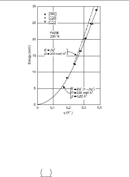
Fig. 7.11. Fe (12 at. % Si) room-temperature spin-wave dispersion relations at low energy. Reprinted with permission from Lynn JW, Phys Rev B 11(7), 2624 (1975). Copyright 1975 by the American Physical Society
where
and a is the lattice spacing. The reality of spin-wave dispersion has been shown by inelastic neutron scattering. See Fig. 7.11.
Specific Heat of Spin Waves (A) With
ai†ai
<< 1, ka << 1, H = 0,
S
and assuming we have a monatomic lattice, the magnons were found to have the energies
7.2 Origin and Consequences of Magnetic Order |
401 |
|
|
where C is a constant. Thus apart from notation (7.161) and (7.193) are identical. We also know that the magnons behave as bosons. We can return to (7.158), (7.159), (7.160), and (7.161) to evaluate the magnetization as well as the internal energy due to spin waves.
Now in (7.158) we can replace a sum with an integral because for large N the number of states is fairly dense and in dk per unit volume is dk/(2π)3. So
∑k |
|
|
1 |
|
→ |
V |
|
∫ |
|
|
|
|
dk |
|
|
|
exp(JSk |
2 |
a |
2 |
|
(2π) |
3 |
|
exp(JSk |
2 |
a |
2 |
/ kBT ) −1 |
|
|
|
/ kBT ) −1 |
|
|
|
|
|
|
|
|
|
|
|
|
V |
|
|
∞ |
|
|
k 2dk |
|
|
|
|
|
|
→ |
|
∫0 |
|
. |
|
|
|
|
|
|
(2π)3 |
exp(JSk 2a2 / kBT ) −1 |
Also we have used that at low T the upper limit can be set to infinity without appreciable error. Changing the integration variable to x = (JS/kBT)1/2ka, we find at low temperature
∑k
where
Similarly
∑k
where
|
1 |
|
|
→ V |
|
exp(JSk 2a2 / kBT ) −1 |
|
(2π)3 |
|
|
∞ |
|
x2dx |
|
N1 |
= ∫ |
|
|
|
|
exp(x2 ) −1 |
|
|
0 |
|
JSk 2a2 |
|
|
→ |
V |
|
exp(JSk 2a2 / kBT ) −1 |
(2π)3 |
|
|
|
|
∞ |
|
x4dx |
|
N2 |
= ∫ |
|
|
|
|
exp(x2 ) −1 |
|
|
0 |
N1 and N2 are numbers that can be evaluated in terms of gamma functions and Riemann zeta functions. We thus find
|
N |
|
|
V |
|
k |
|
|
3 / 2 |
|
|
|
|
|
|
B |
|
N1T 3/ 2 |
|
|
M = |
|
gμBS 1 |
− |
|
|
|
|
|
|
, |
V |
|
|
|
|
|
|
|
2π 2SN JSa2 |
|
|
|
|
|
|
|
|
|
|
|
|
|
|
|
|
|
|
and
|
S 2 Jz |
|
V |
|
k |
B |
5 / 2 |
N T 5 / 2 . |
u = − |
|
+ |
|
|
|
|
|
|
|
|
|
2 |
|
|
|
|
|
|
2 |
|
|
2π 2 N JSa2 |
|
|
402 7 Magnetism, Magnons, and Magnetic Resonance
Thus, from (7.195) by taking the temperature derivative we find the lowtemperature magnon specific heat, as first shown by Bloch, is
Similarly, by (7.194) the low-temperature deviation from saturation goes as T3/2. these results only depend on low-energy excitations going as k2.
Also at low T, we have a lattice specific heat that goes as T3. So at low T we have
CV = aT 3/ 2 + bT 3 , where a and b are constants. Thus
CV T −3/ 2 = a + bT 3 / 2 ,
so theoretically, plotting CT–3/2 vs T3/2 will yield a straight line at low T. Experimental verification is shown in Fig. 7.12 (note this is for a ferrimagnet for which the low-energy ωk is also proportional to k2).
At higher temperatures there are deviations from the 3/2 power law and it is necessary to make refinements in the above theory. One source of deviations is spin-wave interactions. We also have to be careful that we do not approximate away the kinematical part, i.e. the part that requires the spin-deviation quantum number on a given site not to exceed (2Sj + 1). Then, of course, in a more careful analysis we would have to pay more attention to the geometrical shape of the Brillouin zone. Perhaps our worst error involves (7.191), which leads to an approximate density of states and hence to an approximate form for the integral in the calculation of CV and M.
|
200 |
|
|
|
|
|
|
|
|
|
|
5/2deg) |
|
|
|
|
|
|
|
|
|
|
|
–3cm |
100 |
|
|
|
|
|
|
|
|
|
|
3/2(erg |
|
|
|
|
|
|
|
|
|
|
|
|
|
|
|
|
Sample 1 |
|
|
|
K |
|
|
|
|
|
|
|
|
|
|
|
V |
|
|
|
|
|
|
|
|
|
|
|
C |
|
|
|
|
|
|
|
|
|
|
|
|
0 0 |
1 |
2 |
3 |
4 |
5 |
6 |
7 |
8 |
9 |
10 |
|
|
|
|
|
T3/2 (deg3/2) |
|
|
|
|
|
Fig. 7.12. CV at low T for ferrimagnet YIG. After Elliott RJ and Gibson AF, An Introduction to Solid State Physics and Applications, Macmillan, 1974, p 461. Original data from Shinozaki SS, Phys Rev 122, 388 (1961))

7.2 Origin and Consequences of Magnetic Order |
403 |
|
|
Table 7.1. Summary of spin-wave properties (low energy and low temperature)
|
Dispersion |
M = Ms – M |
C |
|
relation |
magnetization |
magnetic Sp. Ht. |
|
|
|
|
Ferromagnet |
ω = A1k2 |
B1T 3/2 |
B2T 3/2 |
Antiferromagnet |
ω = A2k |
B2T 2 (sublattice) |
C2T 3 |
Ai and Bi are constants. For discussion of spin waves in more complicated structures see, e.g., Cooper [7.13].
Equation (7.193) predicts that the density of states (up to cutoff) is proportional to the magnon energy to the 1/2 power. A similar simple development for antiferromagnets [it turns out that the analog of (7.193) only involves the first power of |k| for antiferromagnets] also leads to a relatively smooth dependence of the density of states on energy. In any case, a determination from analyzing the neutron diffraction of an actual magnetic substance will show a result that is not so smooth (see Fig. 7.13). Comparison of spin-wave calculations to experiment for the specific heat for EuS is shown in Fig. 7.14.17 EuS is an ideal Heisenberg ferromagnet.
Density of states, arbitrary scale
1.00
0.75
0.50
0.25
0.00 |
5.0 |
10.0 |
15.0 |
20.0 |
0.0 |
Energy, MeV
Fig. 7.13. Density of states for magnons in Tb at 90 K. The curve is a smoothed computer plot. [Reprinted with permission from Moller HB, Houmann JCG, and Mackintosh AR, Journal of Applied Physics, 39(2), 807 (1968). Copyright 1968, American Institute of Physics.]
17A good reference for the material in this chapter on spin waves is an article by Kittel [7.38]
404 7 Magnetism, Magnons, and Magnetic Resonance
Fig. 7.14. Spin wave specific heat of EuS. An equation of the form C/R = aT3/2 + bT5/2 is needed to fit this curve. For an evaluation of b, see Dyson FJ, Physical Review, 102, 1230 (1956). [Reprinted with permission from McCollum, Jr. DC, and Callaway J, Physical Review Letters, 9 (9), 376 (1962). Copyright 1962 by the American Physical Society.]
Magnetostatic Spin Waves (MSW) (A)
For very large wavelengths, the exchange interaction between spins no longer can be assumed to be dominant. In this limit, we need to look instead at the effect of dipole–dipole interactions (which dominate the exchange interactions) as well as external magnetic fields. In this case spin-wave excitations are still possible but they are called magnetostatic waves. Magnetostatic waves can be excited by inhomogeneous magnetic fields. MSW look like spin waves of very long wavelength, but the spin coupling is due to the dipole–dipole interaction. There are many device applications of MSW (e.g. delay lines) but a discussion of them would take us too far afield. See, e.g., Auld [7.3], and Ibach and Luth [7.33]. Also see Kittel [7.38 p471ff], and Walker [7.65]. There are also surface or Damon– Eshbach wave solutions.18
18 Damon and Eshbach [7.17].
7.2 Origin and Consequences of Magnetic Order |
405 |
|
|
7.2.4 Band Ferromagnetism (B)
Despite the obvious lack of rigor, we have justified qualitatively a Heisenberg Hamiltonian for insulators and rare earths. But what can we do when we have ferromagnetism in metals? It seems to be necessary to take into account the band structure. This topic is very complicated, and only limited comments will be made here. See Mattis [7.48], Morrish [68] and Yosida [7.72] for more discussion.
In a metal, one might hope that the electrons in unfilled core levels would interact by the Heisenberg mechanism and thus produce ferromagnetism. We might expect that the conduction process would be due to electrons in a much higher band and that there would be little interaction between the ferromagnetic electrons and conduction electrons. This is not always the case. The core levels may give rise to a band that is so wide that the associated electrons must participate in the conduction process. Alternatively, the core levels may be very tightly bound and have very narrow bands. The core wave functions may interact so little that they could not directly have the Heisenberg exchange between them. That such materials may still be ferromagnetic indicates that other electrons such as the conduction electrons must play some role (we have discussed an example in Sect. 7.2.1 under RKKY Interaction). Obviously, a localized spin model cannot be good for all types of ferromagnetism. If it were, the saturation magnetization per atom would be an integral number of Bohr magnetons. This does not happen in Ni, Fe, and Co, where the number of electrons per atom contributing to magnetic effects is not an integer.
Despite the fact that one must use a band picture in describing the magnetic properties of metals, it still appears that a Heisenberg Hamiltonian often leads to predictions that are approximately experimentally verified. It is for this reason that many believe the Heisenberg Hamiltonian description of magnetic materials is much more general than the original derivation would suggest.
As an approach to a theory of ferromagnetism in metals it is worthwhile to present one very simple band theory of ferromagnetism. We will discuss Stoner’s theory, which is also known as the theory of collective electron ferromagnetism. See Mattis [7.48 Vol. I p250ff] and Herring [7.56 p256ff]. The two basic assumptions of Stoner’s theory are:
1.The ferromagnetic electrons or holes are free-electron-like (at least near the
Fermi energy); hence their density of states has the form of a constant times E1/2, and the energy is
2.There is still assumed to be some sort of exchange interaction between the (free) electrons. This interaction is assumed to be representable by a molecular field M. If γ is the molecular field constant, then the exchange interaction energy of the electrons is (SI)
where μ represents the magnetic moment of the electrons, + indicates electrons with spin parallel, and − indicates electrons with spin antiparallel to M.
406 7 Magnetism, Magnons, and Magnetic Resonance
The magnetization equals μ (here the magnitude of the magnetic moment of the electron = μB) times the magnitude of the number of parallel spin electrons per unit volume minus the number of antiparallel spin electrons per unit volume. Using the ideas of Sect. 3.2.2, we can write
M = μ∫[ f (E − μ0γMμ) − f (E + μ0γMμ)] |
K E dE , |
(7.198) |
|
2V |
|
where f is the Fermi function. The above is the basic equation of Stoner’s theory, with the sum of the parallel and antiparallel electrons being constant. For T = 0 and sufficiently strong exchange coupling the magnetization has as its saturation value M = Nμ. For sufficiently weak exchange coupling the magnetization vanishes. For intermediate values of the exchange coupling the magnetization has intermediate values. Deriving M as a function of temperature from the above equation is a little tedious. The essential result is that the Stoner theory also allows the possibility of a phase transition. The qualitative details of the M versus T curves do not differ enormously from the Stoner theory to the Weiss theory. We develop one version of the Stoner theory below.
The Hubbard Model and the Mean-Field Approximation (A)
So far, except for Pauli paramagnetism, we have not considered the possibility of nonlocalized electrons carrying a moment, which may contribute to the magnetization. Consistent with the above, starting with the ideas of Pauli paramagnetism and adding an exchange interaction leads us to the type of band ferromagnetism called the Stoner model. Stoner’s model for band ferromagnetism is the nonlocalized mean field counterpart of Weiss’ model for localized ferromagnetism. However, Stoner’s model has neither the simplicity, nor the wide applicability of the Weiss approach.
Just as a mean-field approximation to the Heisenberg Hamiltonian gives us the Weiss model, there exists another Hamiltonian called the Hubbard Hamiltonian, whose mean-field approximation gives rise to a Stoner model. Also, just as the Heisenberg Hamiltonian gives good insight to the origin of the Weiss molecular field. So, the Hubbard model gives some physical insight concerning the exchange field for the Stoner model.
The Hubbard Hamiltonian as originally introduced was intended to bridge the gap between a localized and a mobile electron point of view. In general, in a suitable limit, it can describe either case. If one does not go to the limit, it can (in a sense) describe all cases in between. However, we will make a mean-field approximation and this displays the band properties most effectively.
One can give a derivation, of sorts, of the Hubbard Hamiltonian. However, so many assumptions are involved that it is often clearer just to write the Hamiltonian down as an assumption. This is what we will do, but even so, one cannot solve it exactly for cases that approach realism. Here we will solve it within the mean-field approximation, and get, as we have mentioned, the Stoner model of itinerant ferromagnetism.