

Higher_Mathematics_Part_1
.pdfExample 2. Find points of discontinuity of the function
f (x)= |
3 |
|
|
. |
|
1 |
|
||
|
2 + 4 x+1 |
|||
Solution. The given function is determined on all the numerical axis except
for a point |
x = −1. We find the left — and the right-sided limits at this point: |
|
|
|||||||||||||||||||||||||||||||
|
f (−1− 0) = |
lim |
|
|
|
3 |
|
|
|
|
= |
|
|
|
3 |
|
|
= 3 |
; |
|
|
|
|
|
|
|
||||||||
|
|
|
|
|
1 |
|
|
|
|
|
|
|
|
|
|
|
|
|||||||||||||||||
|
|
|
|
|
|
x→−1−0 |
|
|
|
|
|
|
2 |
+ 4−∞ |
2 |
|
|
|
|
|
|
|
|
|
||||||||||
|
|
|
|
|
2 |
+ 4x+1 |
|
|
|
|
|
|
|
|
|
|||||||||||||||||||
|
|
|
|
|
|
|
|
|
|
|
|
|
|
|
|
|
|
|
|
|
|
|
|
|
|
|
||||||||
|
f (−1+ 0) = |
lim |
|
|
|
3 |
|
|
|
= |
|
|
|
3 |
|
|
|
= 0. |
|
|
|
|
|
|
|
|
||||||||
|
|
|
|
|
|
1 |
|
|
|
|
|
+ 4+∞ |
|
|
|
|
|
|
|
|
|
|||||||||||||
|
|
|
|
|
|
|
x→−1+0 |
|
|
|
2 |
|
|
|
|
|
|
|
|
|
|
|
|
|||||||||||
|
|
|
|
|
|
|
|
2 |
+ 4x+1 |
|
|
|
|
|
|
|
|
|
|
|
|
|
|
|
|
|
|
|
||||||
Thus, |
x = −1 is a point of essential dis- |
|
|
|
|
|
|
|
3 |
|
|
|
|
|
|
|
|
|
|
|||||||||||||||
|
|
|
|
|
|
|
|
|
|
|
|
|
|
|
|
|
||||||||||||||||||
continuity (of the first kind). |
|
|
|
|
|
|
|
|
|
|
|
|
|
|
|
|
|
|
|
|
|
|
|
|
|
|
|
|
|
|
||||
lim f (x) = lim |
|
3 |
|
|
= |
3 |
= |
1. |
|
|
|
|
|
|
|
|
|
|
|
|
|
|
|
|
|
|
|
|
|
|
|
|||
|
1 |
|
2 + 40 |
|
|
|
|
|
|
|
|
|
|
|
1 |
|
|
|
|
|
|
|
|
|
|
|||||||||
x→±∞ |
x→±∞ |
|
|
|
|
|
|
|
|
|
|
|
|
|
|
|
|
|
|
|
|
|
|
|
|
|
|
|
||||||
|
|
|
|
|
|
|
|
|
|
|
|
|
|
|
|
|
|
|
|
|
|
|
|
|
|
|
||||||||
|
2 |
+ 4 |
x+1 |
|
|
|
|
|
|
|
|
|
|
|
|
|
|
|
|
|
|
|
|
|
|
|
|
|
|
|
|
|
|
|
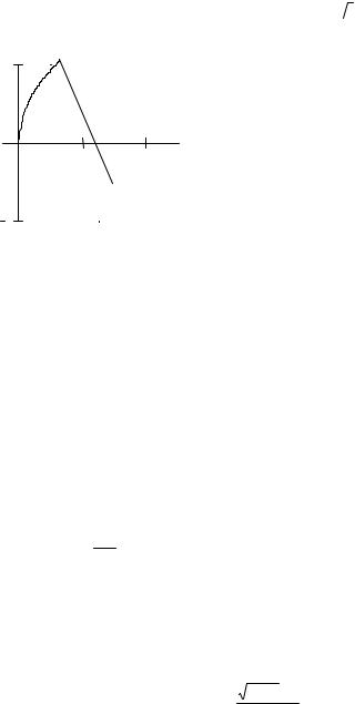
The graph of the function |
f (x) |
is rep- |
|
|
|
|
|
|
|
|
|
|
|
|
|
|
|
|
|
|||||||||||||||
|
|
|
|
|
|
|
|
|
|
|
|
|
|
|
|
|
|
|||||||||||||||||
–2 |
–1 |
|
|
|
0 1 |
2 |
3 |
|||||||||||||||||||||||||||
resented on Fig. 3.12. |
|
|
|
|
|
|
|
|
|
|
|
|
|
|
|
|
|
|
|
|
|
–1 |
|
|
|
|
|
|
|
|
|
|
||
|
|
|
|
|
|
|
|
|
|
|
|
|
|
|
|
|
|
|
|
|
|
|
|
|
|
|
|
|
|
|
||||
Example 3. Find points of discontinuity |
|
|
|
|
|
|
|
|
Fig. 3.12 |
|
|
|
|
|
||||||||||||||||||||
of the function and sketch its graph: |
|
|
|
|
|
|
|
|
|
|
|
|
|
|
|
|
|
|
|
|
|
|||||||||||||
|
|
|
|
|
|
|
|
|
|
|
|
|
|
|
|
|
|
|
|
|
|
|
|
|
|
|
||||||||
|
|
|
|
|
|
|
2 |
x |
if |
0 ≤ x ≤ 1 |
|
|
|
|
|
|
|
|
|
|
|
|
||||||||||||
|
|
|
f (x) |
|
|
4 − 2x, if |
1 < x < 2,5 |
|
|
|
|
|
|
|
|
|
||||||||||||||||||
|
|
|
= |
|
|
|
|
|
|
|
|
|
||||||||||||||||||||||
|
|
|
|
|
|
2x − 7, |
if |
2,5 ≤ x ≤ ∞ |
|
|
|
|
|
|
|
|
|
|||||||||||||||||
|
|
|
|
|
|
|
|
|
|
|
|
|
|
|
|
|
|
|
|
|
|
|
|
|
|
|
|
|
|
|
|
|
|
|
Solution. A function f (x) |
is determined for all values |
|
x ≥ 0. |
But it does |
||||||||||||||||||||||||||||||
not mean that it is continuous for x ≥ 0, |
as far as this function is not elementary. |
|||||||||||||||||||||||||||||||||
It is given by three different formulas for different intervals of changing the argument x and can have discontinuities at points where its analytical expression varies, i.e. at x = 1, x = 2,5. At all other points of the domain of
definition the function f (x) is continuous so as any of three formulas represents
an elementary function, continuous in the interval of changing the argument x. Let us study the behavior of the function at the points x = 1 and x = 2,5 :
lim |
f (x) = lim 2 x = 2 . |
lim |
f (x) = lim (4 − 2x) = 2 . |
x→1−0 |
x→1−0 |
x→1+0 |
x→1+0 |
191
 1
1 


Micromodule 17
BASIC THEORETICAL INFORMATION
DERIVATIVE
The derivative, its geometrical and physical concept. Differentiability and continuity. The rules of differentiation. The derivatives of the elementary functions. The derivative of composite function (The chain rule for differentiation).
Literature: [2, chapter 4], [3, chapter 4, items 4.1—4.2], [4, part 5], [6, chapter 5, §§ 1, 2], [7, chapter 6, § 16], [9, chapter 4, § 2, 4, 5], [10, chapter 4, § 1], [11, chapter 3, §§ 1—15], [8].
17.1. Some problems leading to understanding of the derivative definition
1. The instantaneous velocity of non-uniform motion. Suppose that a body begins to move at the moment of time t = 0 along the straight line. Let the path
traveled by the body over the time t is defined by the formula S = f (t) . A
function S= (f )t is called the law of body motion. Let us consider a path |
|||
traveled by the body over the time [t;t + |
t] ; it is equal to |
||
S = f (t + t) − f (t) . |
|||
If the body is moving uniformly, the ratio of the covered path to the time |
|||
S = |
f (t + t) − f (t) |
|
|
t |
|
t |
|
is velocity. It does not depend on t and t . In case of non-linear motion this |
|
ratio depends both on the chosen time t and on increment |
t and expresses the |
average velocity of motion over the time interval [t; t + t] |
. The less is the time |
interval t , the more reasons we may have to consider the motion over the time t and t + t to be uniform.
The limit
lim |
S |
= lim |
f (t + |
t) − f (t) |
= v(t) , |
t |
|
t |
|||
t→0 |
t→0 |
|
|||
if it exists, is called the instantaneous velocity at the instant of time t .
2. The rate of the chemical reaction. Suppose the chemical reaction begins at an instant of time t . Let us designate the quantity of substance, which reacted
till the instant of time t is c(t) . The quantity of substance, which started to react during time interval [t; t + t] , equals c(t + t) − c(t). The ratio
196

c(t + t) − c(t)
|
|
|
t |
|
|
|
defines the average rate of the reaction and the limit |
|
|||||
lim |
c(t + |
t) − c(t) |
|
|
||
|
t |
|
||||
t→0 |
|
|||||
is called the rate of the chemical reaction at an instant of time t . |
||||||
17.2. The definition of the derivative |
|
|||||
Let any function y = f (x) be defined at the interval |
(a, b) . We take any |
|||||
meaning of x within this interval and apply it to increment |
x . The difference |
|||||
y = f (x + x) − f (x)
is called the increment of a function at point x. The increment of argument x ≠ 0 may gain both positive and negative meanings but the meaning x + x
does not go beyond the limits of the domain of the function f (x) .
Definition 3.19. The limit of the ratio of the |
increment of a function |
|||
y = f (x + x) − f (x) to the increment of argument |
x , when the later tends |
|||
to zero, is called the derivative of a function y = f (x) |
at point x , that is, |
|||
|
|
|
|
|
|
y′(x) = lim |
f (x + x) − f (x) |
|
|
|
|
|
|
|
x |
|
|||
|
x→0 |
|
||
|
|
|
|
|
Definition 3.20. A function, which has the finite derivative at point x , is called differentiable at this point.
Notations for derivative: y′(x), f ′(x) (Lagrange’s notation) or dydx , dfdx
(Leibniz’s notation). From the definition of the derivative it follows that the derivative y' (x) at point x is a number. However, if such a number exists for each inner point of the interval (a, b) , the derivative, then, can be considered as a function of a point x from the given interval.
If |
lim |
f (x + |
x) − f (x) |
= ±∞ , the function f (x) has the infinite derivative |
|
x → 0 |
x |
|
|
at point |
x . |
|
|
|
|
|
|
|
197 |
17.3. The geometrical, physical and mechanical concept of the derivative
Let us try to give the geometrical interpretation of the derivative. We’ll consider the graph of a function y = f (x) at the neighbourhood of point x0 (see
Fig. 3.14). Let P0 be a point of the curve with components (x0 ; f (x0 )) , and P be a point of the graph with components (x0 + x; f (x0 + x)). A straight line, drawn trough the points P0 and P , is called the secant line. If, at the indefinite approach of point P along the graph of a function y = f (x) to point P0 , the secant line P0 P approaches some boundary position ( straight line P0 K ), then this boundary position of the secant line is called the tangent line to the curve y = f (x) at the point P0 .
Let α be the angle, which the tangent line forms with the positive direction
of x-axis and β be the angle between the secant line |
P0 P and x-axis. From the |
||||||||
right triangle P0QP it follows that |
|
|
|
|
|
||||
tgβ = |
PQ |
= |
y |
= |
f (x0 + x) − f (x0 ) |
. |
|||
|
|
x |
|
||||||
|
P Q |
|
|
x |
|
|
|||
|
0 |
|
|
|
|
|
|
|
|
There exists such a limit that |
|
|
|
|
|
|
|||
y′(x0 ) = lim |
|
f (x0 |
+ x) − f (x) |
= lim |
tg β = tg α. |
||||
|
|
|
|
x |
|
||||
x→0 |
|
|
( p→ p0 ) |
||||||
|
|
|
|
|
|
|
x→0 |
|
|
The geometrical concept of the derivative is follows: the derivative of a function y = f (x) at pointі x0 equals the slope of the tangent line to the graph
of a given function at the respective point, that is,
|
|
|
f ′(x0 ) = tgα, |
|
|
|
where |
α is the angle, which is formed by the tangent line to the graph of the |
|||||
function with positive direction of x-axis at point x0 . |
|
|||||
The equation of the tangent line drawn to the graph of a function |
y = f (x) |
|||||
at point P0 (x0 , y0 ) looks as follows |
|
|||||
|
|
|
|
|
||
|
|
y − y0 = f ′(x0 )(x − x0 ), |
|
(3.8) |
||
where |
y0 = f (x0 ) . |
|
||||
198 |
|
|
|
|
|
|

The straight line that passes through the point of contact, perpendicular to the tangent line is called the normal line (it is the straight line P0 N in Fig. 3.14).
The equation of the normal line is
|
|
y − y0 |
= − |
1 |
(x − x0 ). |
|
(3.9) |
|
|
|
f '(x0 ) |
|
|||||
|
|
|
|
|
|
|
|
|
If a function y = f (x) |
describes some physical process, the derivative y′, |
|||||||
then, is the rate of change of this process. This is the way |
the physical concept |
|||||||
of derivative may be interpreted. |
|
|
|
|
y = f (x) could express, |
|||
In other words, whatever dependence a function |
|
|||||||
the ratio |
y can be considered as the average rate of change of a function y |
|||||||
|
x |
x, and the derivative f ′(x) — as the instantaneous |
||||||
with respect to the argument |
||||||||
rate of change of this function. |
|
|
|
|
|
|
||
|
у |
N |
|
|
|
y = f(x) |
||
|
|
|
|
P |
||||
|
f(x0 + x) |
|
|
|
|
|
|
|
|
|
|
|
|
|
К |
|
|
|
|
|
|
|
|
|
|
|
|
f(x0) |
|
|
P0 |
|
Q |
|
|
|
|
|
|
|
|
|||
|
О |
α |
β |
x0 |
x |
|
|
х |
|
|
|
x0 + |
|
x |
|||
|
|
|
Fig. 3.14 |
|
|
|
|
|
The mechanical concept of the derivative. If S = S(t) is the law of motion of a material point (it means that the dependence of the traversed path S on t is given), the derivative S′(t) , then, is velocity v of a point at moment t ; the second derivative S′′(t) is the instantaneous acceleration a of a point at moment t and the third derivative S ′′′(t) is a jerk of a point at moment t , that is,
v = S′(t), a = S′′(t) = v′(t), j = S′′′(t) = v′′(t) = a′(t).
199
17.4. The main rules of differentiation
Let functions u(x), v(x), w(x) be differentiable at point хand С is a constant. Then
|
1. (u + v)′ = u′ + v′ . |
|
2. (u − v)′ = u′ − v′ . |
|
|
|
|
|
|||||||||||||||||||||||||||
|
3. (uv)′ = u′v + uv′ . |
|
4. (Cu)′ = Cu′ . |
|
|
|
|
|
|
|
|
||||||||||||||||||||||||
|
u ′ |
|
|
|
|
u′v − uv′ |
|
6. (uvw)′ = u′vw + uv′w + uvw′ . |
|||||||||||||||||||||||||||
|
5. |
|
|
= |
|
|
|
|
|
|
|
|
|
|
|
|
(v ≠ 0) . |
|
|||||||||||||||||
|
|
|
|
|
|
v |
2 |
|
|
|
|||||||||||||||||||||||||
|
v |
|
|
|
|
|
|
|
|
|
|
|
|
|
|
|
|
|
|
|
|
|
|
|
|
|
|
|
|
|
|
||||
|
|
|
|
|
|
|
|
|
|
|
|
|
|
|
|
|
|
|
17.5. The table of derivatives |
|
|
|
|
|
|
|
|
|
|
|
|||||
|
|
|
|
|
|
(differentiation of the elementary functions table) |
|||||||||||||||||||||||||||||
|
|
|
|
|
|
|
|
|
|
|
|
|
|
|
|
|
|
|
|
|
|
|
|
|
|
|
|
|
|
|
|
|
|
|
Table 17.1 |
|
1. (C)′ = 0 |
|
|
|
|
|
|
|
|
|
|
|
2. (xn )′ = nxn−1 |
|
|
|
|
|
|||||||||||||||||
|
3. ( x)′ = |
1 |
|
|
|
|
|
|
|
|
|
|
|
|
1 ′ |
|
|
1 |
|
|
|
|
|
|
|
|
|||||||||
|
|
|
|
|
|
|
|
|
|
|
|
|
|
|
|
|
|
|
|
|
|
|
|
||||||||||||
|
|
|
|
|
|
|
2 |
|
|
x |
|
|
|
|
|
|
4. |
= − |
x2 |
|
|
|
|
|
|
|
|
||||||||
|
|
|
|
|
|
|
|
|
|
|
|
|
|
|
x |
|
|
|
|
|
|
|
|
|
|||||||||||
|
5. (ax )′ = ax ln a |
|
|
|
|
|
|
6. (ex )′ = ex |
|
|
|
|
|
|
|
|
|
||||||||||||||||||
|
7. (log |
a |
x)′ = |
|
1 |
|
|
|
|
|
|
8. (ln x)′ = |
1 |
|
|
|
|
|
|
|
|
|
|||||||||||||
|
x ln a |
|
x |
|
|
|
|
|
|
|
|
|
|||||||||||||||||||||||
|
|
|
|
|
|
|
|
|
|
|
|
|
|
|
|
|
|
|
|
|
|
|
|||||||||||||
|
9. (sin x)′ = cos x |
|
|
|
|
|
|
10. (cos x)′ = − sin x |
|||||||||||||||||||||||||||
|
11. (tg x) |
′ |
|
|
|
|
|
|
1 |
|
|
|
|
|
|
|
|
|
|
|
|
|
1 |
|
|
|
|
||||||||
|
= cos2 x |
|
12. (ctg x)′ = − sin2 x |
||||||||||||||||||||||||||||||||
|
|
|
|||||||||||||||||||||||||||||||||
|
13. (arcsin x)′ = |
|
1 |
|
|
|
14. |
(arccos x)′ |
= − |
1 |
|
|
|||||||||||||||||||||||
|
|
1− x2 |
|
|
|
|
|
|
|||||||||||||||||||||||||||
|
|
|
1− x2 |
||||||||||||||||||||||||||||||||
|
|
|
|
|
|
|
|
|
|
|
|
|
|
|
|
|
|
|
|
|
|
|
|
|
|
||||||||||
|
15. (arctg x)′ |
= |
|
|
1 |
|
|
|
16. |
(arcctg x)′ |
= − |
1 |
|
|
|||||||||||||||||||||
|
1+ x2 |
|
|
1+ x2 |
|
||||||||||||||||||||||||||||||
|
17. (sh x)′ = ch x |
|
|
|
|
|
|
18. (ch x)′ = sh x |
|
|
|
|
|
||||||||||||||||||||||
|
19. (th x)′ |
= |
|
1 |
|
|
|
|
|
|
|
|
|
(cth x)′ |
|
|
|
1 |
|
|
|
|
|
||||||||||||
|
|
|
|
|
|
|
|
20. |
= − |
|
|
||||||||||||||||||||||||
|
ch2 x |
|
|
|
|
|
|
||||||||||||||||||||||||||||
|
|
|
|
|
|
|
sh2 x |
||||||||||||||||||||||||||||
|
|
|
|
|
|
|
|
|
17.6. The derivative of the composite function |
||||||||||||||||||||||||||
|
|
|
(The chain rule for differentiation). Table of derivatives |
||||||||||||||||||||||||||||||||
|
If a function |
|
|
y = f (u) has the derivative at point u , and a function u = g(x) |
|||||||||||||||||||||||||||||||
has the derivative at point x , a |
composite |
function |
y = f (g(x)) then is |
||||||||||||||||||||||||||||||||
differentiable at point |
x . In this case |
|
|
|
|
|
|
|
|
|
|
|
|
||||||||||||||||||||||
200 |
|
|
|
|
|
|
|
|
|
|
|
|
|
|
|
|
|
|
|
|
|
|
|
|
|
|
|
|
|
|
|
|
|
|
|