Добавил:

Upload Опубликованный материал нарушает ваши авторские права? Сообщите нам.

Вуз:

Национальный авиационный университет

Предмет:

[НЕСОРТИРОВАННОЕ]

Файл:

Higher_Mathematics_Part_1

.pdf

Скачиваний:

1052

Добавлен:

19.02.2016

Размер:

6.63 Mб

Скачать

☆

<<< < Предыдущая 4 5 6 7 8 9 10 11 12 13 14 1516 / 2816 17 18 19 20 21 22 23 24 25 26 27 28 > Следующая >>>

12.24. а)

lim

(2n − 3)3 + 7n3

;

3(3n − 1)3

n→∞

lim

2 + 5 + 8 + ... + (3n − 1)

;

n→∞

n (4n + 2)(n + 11)

12.25. а)

lim

(2n − 5)(n + 1)(3n − 1)

;

n→∞

(4n − 1)3

lim

3 + 5 + 7 + ... + (2n + 1)

;

n→∞

(n + 1)

2n + 3

12.26. а)

lim

(3n + 1)(n − 1)(2n − 3)

;

n→∞

(n + 2)3

lim

3 + 6 + 9 + ... + 3n

;

n→∞

n + 3

12.27. а)

lim

(n + 2)(2n − 1)(2n + 3)

;

n→∞

(2n + 5)3

lim

3 + 7 + 11+ ... + (4n − 1)

;

2 + 6 + 10 + …+ (4n − 2)

n→∞

12.28. а)

lim

(n + 4)(3n − 1)(2n + 1)

;

n→∞

(n + 1)(2n + 3)2

lim

1+ 5 + 9 + ...+ (4n − 3)

;

n→∞

2 + 5 + 8 + …+ (3n − 1)

12.29. а)

lim

(n − 3)(2n − 3)(n + 2)

;

n→∞

(n + 4)(2n + 7)2

lim

3 + 5 + 7 + ... + (2n + 1)

;

n→∞

2 + 4 + 6 + …+ 2n

12.30. а)

lim

(3n − 1)(2n −1)(n − 1)

;

(n + 2)(2n + 3)2

n→∞

lim

...+

4n − 3

;

n→∞

		n + 1 + 6 n5
b) lim				;
	4	n3 + 7
n→∞			3n4

lim

(n + 5)!+ (n + 4)! .

n→∞

(n + 5)!− (n + 3)!

6 n7 + n

lim

;

n3 + 3

n→∞

4n4

lim

(n + 6)!+ (n + 4)! .

n→∞

(n + 6)!− (n + 5)!

3 n2 + n

lim

;

n3 + 3 8n4

n→∞

lim

(n + 2)!+ (n + 1)!

n→∞

(n + 2)!+ n!

3 n5 + n

lim

;

n8 + 3

27n4

n→∞

lim

2(n + 2)!+ (n + 1)!

n→∞

3(n + 2)!− n!

lim

4 n9 + n 5

;

n8 + 6

n13

n→∞

lim

(n + 3)!+ (n + 2)!

n→∞

10(n + 2)!− (n + 1)!

4 n + n

lim

;

n2 + 7

n→∞

lim

(n + 4)!+ (n + 3)!

n→∞ n(n + 3)!− (n + 2)!

lim

(n + 1)(n + 1)!+ (n + 2)!

;

n(n + 1)!− (n + 2)!

n→∞

lim

5 n2 + n8

n2 + 7

n→∞

151

Micromodule 13

BASIC THEORETICAL INFORMATION

THE CONCEPT OF A FUNCTION. CLASSIFICATION

OF FUNCTIONS. LIMIT OF A FUNCTION.

THEOREMS ABOUT LIMITS

The Concept of a function.

Elementary functions and their graphs.

13.1. The concept of a function

Definition 3.5. If to each value of a variable x which belongs to a set of real

numbers D there corresponds by a certain rule the definite value of			y which
belongs to a set of real numbers		E then y is said to be a function of	x. Thus,
we write y = f (x)	or f :D → E. The element x D is said to be an argument
of the function f ,	the element	y E is the value of the function f correspon-
ding to the element	x D .

Definition 3.6. The set D is called a domain of definition of the function f (x) , and the set E is a range (or the set of values) of the function f (x) .

Different ways of functions representation are possible:

1.analytical method (by means of the formula);

2.tabular method (by means of a table where numerical values of an independent variable and values of a function corresponding to them) had written;

3.graphic method.

For the graphic method we consider variables x and y as Cartesian coordinates of a point on a plane. In this case the graph of a function is a set of points

on	a coordinate plane x0y , whose	abscissas are independent variables, and
ordinates are corresponding values of the function.
	Definition 3.7. If the function reflects the set		D into the set E so that for
any	x1 and x2 D provide x1 ≠ x2 ,	f (x1) ≠ f (x2 )	then a function of x = ϕ( y)
which reflects the set E into the set		D is said to be an inverse to the function

f (x). To find a function inverse to the given y = f (x), it is necessary to express x from this equality through y . By tradition, a function inverse to y is denoted so: y = ϕ(x).

If the functions y = f (x) and x = ϕ( y) are mutually inversed, their graphs

are expressed by the same curve. But, if we denote again an argument of the inverse function through x, and a function through y the graphs of the func-

tions y = f (x) and y = ϕ(x) will be symmetric relatively bisectors of the first and the third coordinate angles.

152

The domain of definition D of a function y = f (x) is a set of those numbers

that the argument of the function can take on and for which the analytical expression of the function is meaningful.

Those are real values of the argument for which:

1.an expression standing in the denominator of a fraction is not equal to

zero;

2.an expression under a square root or a root of an even degree is positive;

3.an expression under the sign of a logarithm is positive;

4.an expression under the sign of arcsine or arccosine does not exceed a unit by the absolute value;

5.the argument of a cotangent is not equal to n π , n Z.

6. the argument of a tangent is not equal to π2 + n π, n Z.

If the given function is the sum of two or the greater number of various functions we find separately a domain of definition of each function, and a common part (intersection) of domains of definition of the functions is the domain of definition of the given function.

Definition 3.8. A function y = f (x) is said to be even if for any value of an argument from a domain of definition the equality f (− x) = f (x) holds. The graph of an even function is symmetric relatively to the axis of ordinates.

Definition 3.9. A function y = f (x) is said to be odd if for any value of an argument from the domain of definition the equality f (− x) = − f (x) holds. The

graph of an odd function is symmetric relatively to the origin of coordinate system.

The function which is neither even, nor odd, is said to be as a general view function.

13.2. Elementary functions and their graphs

The basic elementary functions are the following analytically given functions:

1)a power function y = xα , where α is a real number;

2)an exponential function y = ax , where a is the positive number different

from a unit;	y = loga x , where a is a positive number different
3) a logarithmic function
from a unit;		y = cos x, y = tgx, y = ctgx, y = sec x,
4) trigonometric functions y = sin x,
y = cosecx.		y = arcsin x, y = arccos x, y = arctgx,
5) inverse trigonometric	functions:

y = arcctgx, y = arcsec x, y = arccosecx.

153

Let us consider domains of definition and graphs of the basic elementary

functions.

1. A power function is

y = xα . If

α Q,

i.e. α =

, where

m N,

n N.

The integer α can be considered as a special case of a fraction if n =1.

For α > 0 and even n a domain of definition of the function

y = xα

will be

an infinite interval [0; + ∞ ) , for odd

n the domain of definition of the function

is an infinite interval ( − ∞; + ∞ ) .

For even m a power function is even, for

m and n simultaneously odd a

power function is odd, and for even

n the power function is neither even

nor odd.

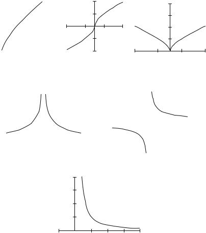
Graphs of power functions for some values of α > 1

are represented on

Fig. 3.1 (a)

y = x3 , b) y = x2 , c)

y = x3 ).

Graphs of the power function

y = xα for 0 < α < 1 are represented on

Fig. 3.2 (a)

y = x4 , b) y = x5 , c)

y = x3 ).

If α < 0,

x = 0

does not enter into a domain of definition of a power function

y = xα .

Graphs of function y = xα at

α < 0

are represented on Fig. 3.3 (a) y = x− 5 ,

y = x

−

5 , c) y = x

2 ).

If a power function is even for α > 0 the range of this function is an infinite

interval [0; + ∞ ),

and for α < 0 is an interval (0; + ∞ ).

–3

–1 –1

–3

–1

–3

–1

Fig. 3.1

154

3							2								4
3							2

2							1								3
2															3
1						–3	–1	1		3					2
						–3	–1	1		3
							–1								1
							–1								1
							–2								1	3
–1	1		3	5			–2				–3			–1
–1	1		3	5							–3			–1
a						b					c
							Fig. 3.2
				3							3
											3
											1
				2
				2


				1				–3			–1 –1		1			3


												–3
		–1		0		1
		–1		0		1
		a							b
						4
						3
						2
						1
					–1	0	1	2		3	4
					c
							Fig. 3.3
	If a power function is odd for						α > 0 the range of this function is an interval

(−∞; ∞ ) , and for α < 0 is a union of intervals (−∞; 0) (0; + ∞ ).

If a power function is neither even nor odd for	α > 0 the range of the
function is the interval [ 0; + ∞ ), for α < 0 is (0; + ∞ ).
2. Let’s consider the exponential function y = ax ,	where а is a positive

number different from unit. The domain of definition of an exponential function

155

y = ax is the set of all real numbers, i.e. x R, and the range of this function is the set of positive numbers, i.e. y (0; + ∞) . Graphs of exponential function for α > 1

(a = 2) and for 0 < a <1 (a = 12 )							are represented on Fig. 3.4 (a) y = 2x , b)								y = (	1	)x ).
(a = 2) and for 0 < a <1 (a = 12 )							are represented on Fig. 3.4 (a) y = 2x , b)								y = (	2	)x ).
			4								4
			4								4
			3								3
			3								3
			2								2
			2								2
			1								1
			1								1


–3	–2	–1		0	1	2	3	–3	–2	–1		0	1	2	3
a								b
								Fig. 3.4
3. A logarithmic function is								y = loga x, where a is a positive number

different from unit. The domain of definition of the logarithmic function y = loga x is the set of positive numbers (0; + ∞ ), and the range of the function is the set of all real numbers. Graphs of logarithmic function are represented on

Fig. 3.5 (a) y = log2 x , b)

y = log1 x ).

–1

0,5

1,5

–1

0,5

1,5

–3

Fig. 3.5

4. Trigonometric functions. The domain of definition of functions

y = cos x

and y = sin x

is the set of all real numbers, the domain of functions y = tgx and

y = sec x

is the set of real numbers which are not equal to

+ kπ,

k Z and

the domain of definition of functions y = ctg x

and

y = cos ec x is the set of real

numbers which are not equal to kπ, k Z.

156

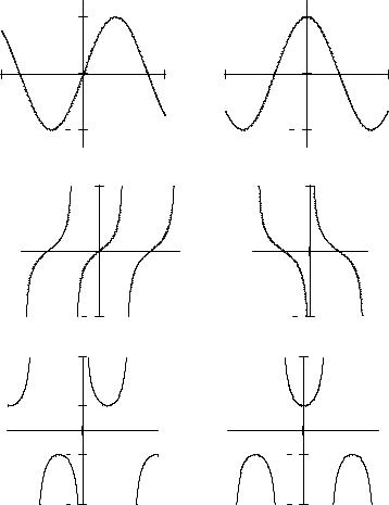
The range of functions	y = cos x and	y = sin x is the interval	[	]	the
				−1; 1 ,
range of functions y = tgx	and y = ctg x	is the set of all real numbers, and the

set	of values	of functions			y = sec x and		y = cos ec x	is	unions of		intervals
(−∞; − 1] [1, + ∞ ). Graphs of trigonometric functions:									y = sin x;	y = cos x;
y = tg x; y = ctg x;			y = cos ecx; y = sec x			are represented on Fig. 3.6 (a)					y=sin x,
b)	y = cos x ,	c) y = tgx ,		d)	y = ctg x, e)	y = cos ecx , f)		y = sec x ).
			1					1
			1					1
	a						b
			5					5
			0						0
			5					5
	c						d
			3					3
			1					1
			0					0
			1					1
	e		3				f	3
	e						f

Fig. 3.6

157

5. Inverse trigonometric functions. The domain of definition of the functions y = arcsin x and y = arccos x is the interval [−1; 1] , the domain of definition of

functions y = arctgx and y = arcctgx is the set of all real numbers, the domain of definition of functions y = arcsecx and y = arccosecx is the union of intervals

( − ∞ ; − 1] [1; + ∞ ).
The range of the function	y = arcsin x	is the interval	−	π	;	π	, the range of
	[0, π] , the			2		2
y = arccos x is the interval	[0, π] , the	range of y = arctgx				is	the interval

−

y = arcctgx

;

, the range of

the

−

y =

arccosecx is the set

of intervals

;

y = arcsecx is the set of intervals 0;

π2

;

interval		(0; π) ,		the	range of
0	0;	π	, and	the	range of
		2

π.

Graphs of inverse trigonometric functions y = arcsin x (а); y = arccos x; y =

= arctg x (в); y = arcctg x (c); y = arccosec x (d); y = arcsec x (е) are represented on Fig. 3.7.

Definition 3.10. A function is said to be periodic with the period T (where T is a number which is not equal to zero) if for any argument x from the

domain of definition of the function	x + T and x − T belong to the domain of
the function and f (x + T ) = f (x) or	f ( x − T ) = f (x).

The period of a function is the least of all positive periods (if such exists). In this case all periods of a function are multiples to the least period T = kT0 ,

where T0 is the least positive period of the function, and k			is an integer not
equal to zero.			y = cosec x is the
The period of the functions y = sin x,	y = cos x,	y = sec x,	y = cosec x is the
number 2π, and the period of the function	y = sin ax	is the number T =		2π	.
				a

Definition 3.11. The function received from the basic elementary functions by means of a finite number of algebraic operations and a finite number of formation of composite functions is said to be an elementary function.

Functions may be algebraic and transcendental.

Algebraic functions consist of:

— the whole rational function or a polynomial

y = a0 xn + a1xn−1 + ...+ an−1x + an , where n is a whole positive number;

158

— a rational function which is expressed by a ratio of two polynomials:

y = a0 xn + a1xn−1 +...+ an−1x + an ; b0 xm + b1xm−1 +...+ bm−1x + bm

— an irrational function which is written as an expression containing the variable x under the sign of radicals.

–2	–1	0	1	2	–2	–1	0	1	2
a					b
a					b

–2

–3

–2

–1

–3

–2

–1

–2

Fig. 3.7

Definition 3.12. A function

y = f (x) is said to be algebraic if it satisfies the

equation

A0 (x) yn + A1 (x) yn−1 +...+ An−1 (x) y + An (x)= 0 ,

where A0 (x), A1 (x), ..., An (x)

are whole rational functions of

A0 (x)≠ 0; n

is a whole positive number.

159

Functions which are not algebraic are said to be transcendental. For example, y = loga x, y = tgx, y = arcsin x.

Transformations of graphs of functions. If the graph of a function y = f (x) is known: then

а) the graph of the function y1= − f (x) is a mirror reflection of the graph of the function y = f (x) with respect to the axis Ox;

b) the graph of the function y 2= f (− x) is the mirror reflection of the graph

of the function with respect to the axis Oy;
c) the	graph of the function y3 = f (x − a) is a graph	of the	function
y = f (x)	which moves on a units to the right along the axis	Ox (for	a < 0 a

removal occurs to the left along the axis Ox );

d) ordinates of the graph of the function y4 = A f (x) for identical values x are increased ordinates of the function y = f (x) in A times (if A < 1 length

of ordinates are reduced in A times in comparison with the graph of						y = f (x) );
e) the graph		of	the function y5	= f (a x) is compressed for		a	>1 and

stretched for	a	<1	along the axis	Ox in a times. If a function	y = f (x) is

periodic with the period T , the period of a function y = f (a x) is decreased in a times for a > 1 and increased for 0 < a < 1;

f) the graph of function y6 = f (x) + B moves along the axis Oy on B units of scale (for B > 0 upward and for B < 0 downward).

13.3. Limit of a function

Suppose a function y = f (x) is defined at the some neighbourhood of a point а, except may be, the point а.

Number A is called a limit of a function y = f(x) if x→ a, if for any very small number ε > 0 such number δ = δ(ε) > 0 may be found, that for any x

such as х–a <δ, х≠a, the following inequality is fulfilled f (x) − A < ε.

We denote it as:

lim f (x) = A or f (x) → A if x → a .

x→a

160

<<< < Предыдущая 4 5 6 7 8 9 10 11 12 13 14 1516 / 2816 17 18 19 20 21 22 23 24 25 26 27 28 > Следующая >>>

Соседние файлы в предмете [НЕСОРТИРОВАННОЕ]

#
05.09.2019478.78 Кб6gtfnmТ.docx
#
15.08.2019637.53 Кб3Gulenko.docx
#
12.11.2018765.44 Кб6Hagakure_-_Sokrytoe_v_listve.doc
#
19.02.20166.95 Mб201Higher Mathematics. Part 3.pdf
#
19.02.20169 Mб95Higher_Mathematics_Part_1.pdf
#
19.02.20166.63 Mб1052Higher_Mathematics_Part_1.pdf
#
19.02.20167.48 Mб408Higher_Mathematics_Part_2.pdf
#
19.02.20169.73 Mб45Higher_Mathematics_Part_2.pdf
#
19.02.20167.31 Mб123Higher_Mathematics_Part_2.pdf
#
19.02.20169.11 Mб304Higher_Mathematics_Part_3.pdf
#
19.02.2016694.82 Кб11HiraganaKatakanaWorkSheet (1).pdf