Добавил:
Опубликованный материал нарушает ваши авторские права? Сообщите нам.
Вуз: Предмет: Файл:

Finkenzeller K.RFID handbook.2003

.pdf
Скачиваний:
232
Добавлен:
23.08.2013
Размер:
6.09 Mб
Скачать

302

10 THE ARCHITECTURE OF ELECTRONIC DATA CARRIERS

Bit line

Data = 0

B


C

Word line


UCC

UCC

Ferroelectric C


Pulse common plate line

D

A


Data = 1

Figure 10.35 FRAM cell structure (1 bit) and hysteresis loop of the ferroelectric capacitor

Table 10.3 Comparison between FRAM and EEPROM (Panasonic, n.d.)


FRAM

EEPROM


µ 2

130

µ

2

Size of memory cell

80 12m

5

m

Lifetime in write cycles

10

10


Write voltage

2 V

12 V


Energy for writing

0.0001 µJ

100

µJ

Write time

0.1 µs

10 ms (10 000 µs)


hysteresis loop. After the removal of the electric field the FRAM cell falls into state D, which recreates the originally stored state A (Haberland, 1996).

Writing a ‘1’ or ‘0’ to the FRAM cell is achieved simply by the application of an external voltage UCC or +UCC. After the voltage is removed the FRAM cell returns to the corresponding residual state A or C.

10.3.4 Performance comparison FRAM – EEPROM

Unlike EEPROM cells, the write operation of a FRAM cell occurs at a high speed. Typical write times lie in the region of 0.1 µs. FRAM memories can therefore be written in ‘real time’, i.e. in the bus cycle time of a microprocessor or the cycle time of a state machine.

FRAMs also beat EEPROMs in terms of power consumption by orders of magnitude. FRAM memory was therefore predestined for use in RFID systems. However, problems in combining CMOS processors (microprocessor) and analogue circuits (HF interface) with FRAM cells on a single chip still prevent the rapid spread of this technology (Table 10.3).

10.4Measuring Physical Variables

10.4.1 Transponder with sensor functions

Battery operated telemetry transmitters in the frequency range 27.125 MHz or 433 MHz are normally used for the detection of sensor data. The fields of application of these

10.4 MEASURING PHYSICAL VARIABLES

303

Address and security logic

HF interface A/D

converter ϑ

EEPROM

ROM

or FRAM


Chip

Figure 10.36 Inductively coupled transponder with additional temperature sensor

systems are very limited, however, and are restricted by their size and the lifetime of the battery.

Specially developed RFID transponders incorporating an additional A/D converter on the ASIC chip facilitate the measurement of physical variables. In principle, any sensor can be used, in which the resistance alters in proportion to physical variables. Due to the availability of miniaturised temperature sensors (NTC), this type of system was first developed for temperature measurement (Figure 10.36).

Temperature sensor, transponder ASIC, transponder coil and backup capacitors are located in a glass capsule, like those used in animal identification systems (see Section 13.6.1). (Ruppert, 1994). The passive RFID technology with no battery guarantees the lifelong functioning of the transponder and is also environmentally friendly.

The measured value of the A/D converter can be read by a special reader command. In read-only transponders the measured value can also be appended to a periodically emitted identification number (serial number).

Nowadays, the main field of application for transponders with sensor functions is wireless temperature measurement in animal keeping. In this application the body temperatures of domestic and working animals are measured for health monitoring and breeding and birth control. The measurement can be performed automatically at feed and watering points or manually using a portable reader (Ruppert, 1994).

In industrial usage, transponders with a sensor function may be used anywhere where physical variables need to be measured in rotating or moving parts where cable connections are impossible.

In addition to the classical temperature sensors a large number of sensors can already be integrated. Due to their power consumption, however, only certain sensors are suitable for passive (battery-free) transponders. Table 10.4 (Bogel¨ et al., 1998) shows an overview of sensors that can be used in active or passive transponders. Solutions that can be realised as a single chip are cheaper.

10.4.2 Measurements using microwave transponders

Industry standard microwave transponders can also be used to measure speed and distance by the analysis of the Doppler effect and signal travelling times (Figure 10.37).

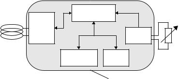
304 10 THE ARCHITECTURE OF ELECTRONIC DATA CARRIERS

Table 10.4 Sensors that can be used in passive and active transponders (mm = micromechanic)

Sensor


Integratable


Passive


Active

Single chip


transponder

transponder

transponder


Temperature


Yes


Yes


Yes

Yes

Moisture


Yes


Yes


Yes

Yes

Pressure


mm


Yes


Yes

Yes

Shock


mm


Yes


Yes


Acceleration


mm


Yes


Light


Yes


Yes


Yes

Yes

Flow


Yes


Yes


PH value


Yes


Yes


Gases


Yes


Yes


Conductivity


Yes


Yes

Yes


v


a


Direction of propagation


Reader


v


Microwave


d


transponder


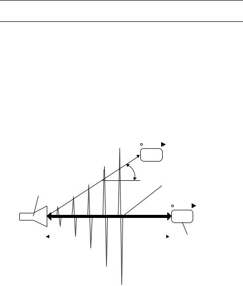
Figure 10.37 Distance and speed measurements can be performed by exploiting the Doppler effect and signal travelling times

The Doppler effect occurs in all electromagnetic waves and is particularly easy to measure in microwaves. If there is a relative movement between the transmitter and a receiver, then the receiver detects a different frequency than the one emitted by the transmitter. If the receiver moves closer to the transmitter, then the wavelength will be shortened by the distance that the receiver has covered during one oscillation. The receiver thus detects a higher frequency.

If the electromagnetic wave is reflected back to the transmitter from an object that has moved, then the received wave contains twice the frequency shift. There is almost always an angle α between the direction of propagation of the microwaves

10.4 MEASURING PHYSICAL VARIABLES

305


Table 10.5 Doppler frequencies at different speeds


fd (Hz)

V (m/s)

V (km/h)


0

0

0


10

0.612

1.123


20

1.224

4.406


50

3.061

9.183


100

6.122

18.36


200

12.24

36.72


500

30.61

110.2


1000

61.22

220.39


2000

122.4

440.6


and the direction of movement of the ‘target’. This leads to a second, expanded Doppler equation:

d =

c

·


f


fTX · 2v


cos α

(10.1)

=

fd · c


v


(10.2)

2fTX · cos α


The Doppler frequency fd is the difference between the transmitted frequency fTX and

the received

frequency f

RX. The relative speed of the object is

v

· cos

α

,

c

is the speed


8


of light, 3 × 10


m/s.


A transmission frequency of 2.45 GHz yields the Doppler frequencies shown in Table 10.5 at different speeds.

To measure the distance d of a transponder, we analyse the travelling time td of a

microwave pulse reflected by a transponder:


d =

1

· td · c

(10.3)

2

The measurement of the speed or distance of a transponder is still possible if the transponder is already a long way outside the normal interrogation zone of the reader, because this operation does not require communication between reader and transponder.

10.4.3 Sensor effect in surface wave transponders

Surface wave transponders are excellently suited to the measurement of temperature or mechanical quantities such as stretching, compression, bending or acceleration. The influence of these quantities leads to changes in the velocity v of the surface wave on the piezocrystal (Figure 10.38). This leads to a linear change of the phase difference between the response pulses of the transponder. Since only the differences of phase position between the response pulses are evaluated, the measuring result is fully independent of the distance between transponder and reader.

A precise explanation of the physical relationships can be found in Section 4.3.4.

306

10

THE ARCHITECTURE OF ELECTRONIC DATA CARRIERS


Force and displacement


ds

Chemical densities


Stretching


Sensitive coating


Compressing


... yields a scaling of the sensor’s


response in time by a factor


Temperature

s = 1 + e,


... the acoustic delay T is changed by ∆t = ε T

Figure 10.38 Influence of quantities on the velocity v of the surface wave in piezocrystal are shear, tension, compression and temperature. Even chemical quantities can be detected if the surface of the crystal is suitably coated (reproduced by permission of Technische Universitat¨ Wien, Institut fur¨ allgemeine Elektrotechnik und Elektronik)

Figure 10.39 Arrangement for measuring the temperature and torque of a drive shaft using surface wave transponders. The antenna of the transponder for the frequency range 2.45 GHz is visible on the picture (reproduced by permission of Siemens AG, ZT KM, Munich)

10.4 MEASURING PHYSICAL VARIABLES

307

Figure 10.40 A surface wave transponder is used as a pressure sensor in the valve shaft of a car tyre valve for the wireless measurement of tyre pressure in a moving vehicle (reproduced by permission of Siemens AG, ZT KM, Munich

The working range of surface wave transponders extends to low temperatures of 196 C (liquid nitrogen) and in a vacuum it even extends to very low temperatures.1 The normal surface wave crystals have only limited suitability for high temperatures. For example, in lithium niobate segregation occurs at a temperature of just 300 C; in quartz there is a phase transition at 573 C. Moreover, at temperatures above 400 C

the aluminium structure of the interdigital transducer is damaged.

However, if we use a crystal that is suitable for high temperatures such as langasite with platinum electrodes, surface wave sensors up to temperatures as high as around 1000 C can be used (Reindl et al., 1998b).

Figures 10.39 and 10.40 show transponders used for measuring physical properties.

1 At very low temperatures, however, the sensitivity S of a SAW transponder ultimately tends towards zero.

RFID Handbook: Fundamentals and Applications in Contactless Smart Cards and Identification, Second Edition

Klaus Finkenzeller Copyright 2003 John Wiley & Sons, Ltd.

ISBN: 0-470-84402-7

11

Readers

11.1Data Flow in an Application

A software application that is designed to read data from a contactless data carrier (transponder) or write data to a contactless data carrier, requires a contactless reader as an interface. From the point of view of the application software, access to the data carrier should be as transparent as possible. In other words, the read and write operations should differ as little as possible from the process of accessing comparable data carriers (smart card with contacts, serial EEPROM).

Write and read operations involving a contactless data carrier are performed on the basis of the master–slave principle (Figure 11.1). This means that all reader and transponder activities are initiated by the application software. In a hierarchical system structure the application software represents the master, while the reader, as the slave, is only activated when write/read commands are received from the application software.

To execute a command from the application software, the reader first enters into communication with a transponder. The reader now plays the role of the master in relation to the transponder. The transponder therefore only responds to commands from the reader and is never active independently (except for the simplest read-only transponders. See Chapter 10).

A simple read command from the application software to the reader can initiate a series of communication steps between the reader and a transponder. In the example in Table 11.1, a read command first leads to the activation of a transponder, followed by the execution of the authentication sequence and finally the transmission of the requested data.

The reader’s main functions are therefore to activate the data carrier (transponder), structure the communication sequence with the data carrier, and transfer data between the application software and a contactless data carrier. All features of the contactless communication, i.e. making the connection, and performing anticollision and authentication procedures, are handled entirely by the reader.

11.2Components of a Reader

A number of contactless transmission procedures have already been described in the preceding chapters. Despite the fundamental differences in the type of coupling

310


11 READERS


Master

Slave


Command


Command


Application

Reader


Trans-


ponder


Response


Response


Master


Slave


Data flow

Figure 11.1 Master–slave principle between application software (application), reader and transponder

Table 11.1 Example of the execution of a read command by the application software, reader and transponder

Application reader

Reader transponder

Comment

BlockreadAddress[00]


Read transponder memory


Request

[address]


Transponder in the field?


ATRSNR[4712]

Transponder operates with


GETRandom

serial number


Initiate authentication


Random[081514]


SENDToken1


GETToken2

Authentication successfully


Read@[00]

completed


Read command [address]

Data[9876543210]

Data[9876543210]

Data from transponder


Data to application

(inductive — electromagnetic), the communication sequence (FDX, HDX, SEQ), the data transmission procedure from the transponder to the reader (load modulation, backscatter, subharmonic) and, last but not least, the frequency range, all readers are similar in their basic operating principle and thus in their design.

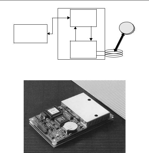
Readers in all systems can be reduced to two fundamental functional blocks: the control system and the HF interface, consisting of a transmitter and receiver (Figure 11.2). Figure 11.3 shows a reader for an inductively coupled RFID system. On the right-hand side we can see the HF interface, which is shielded against undesired spurious emissions by a tinplate housing. The control system is located on the left-hand side of the reader and, in this case, it comprises an ASIC module and microcontroller. In order that it can be integrated into a software application, this reader has an RS232 interface to perform the data exchange between the reader (slave) and the external application software (master).

11.2 COMPONENTS OF A READER


311

Application control commands

Control

Data


(signal coding

carrier


protocol)


Application


(computer with

Received

Transmitted

software

data


data

application)


HF


interface

Antenna


Figure 11.2 Block diagram of a reader consisting of control system and HF interface. The entire system is controlled by an external application via control commands

Figure 11.3 Example of a reader. The two functional blocks, HF interface and control system, can be clearly differentiated (MIFARE reader, reproduced by permission of Philips Electronics N.V.)

11.2.1 HF interface

The reader’s HF interface performs the following functions:

generation of high frequency transmission power to activate the transponder and supply it with power;

modulation of the transmission signal to send data to the transponder;

reception and demodulation of HF signals transmitted by a transponder.

The HF interface contains two separate signal paths to correspond with the two directions of data flow from and to the transponder (Figure 11.4). Data transmitted to

312

11 READERS

Quarz

Oscillator

Modulator

Output

Antenna box


module

Transmission


data


/


Received


/


data


Demodulator

Amplifier

Bandpass filter


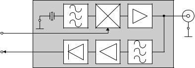
Figure 11.4 Block diagram of an HF interface for an inductively coupled RFID system

the transponder travels through the transmitter arm. Conversely, data received from the transponder is processed in the receiver arm. We will now analyse the two signal channels in more detail, giving consideration to the differences between the different systems.

11.2.1.1Inductively coupled system, FDX/HDX

First, a signal of the required operating frequency, i.e. 135 kHz or 13.56 MHz, is generated in the transmitter arm by a stable (frequency) quartz oscillator. To avoid worsening the noise ratio in relation to the extremely weak received signal from the transponder, the oscillator is subject to high demands regarding phase stability and sideband noise.

The oscillator signal is fed into a modulation module controlled by the baseband signal of the signal coding system. This baseband signal is a keyed direct voltage signal (TTL level), in which the binary data is represented using a serial code (Manchester, Miller, NRZ). Depending upon the modulator type, ASK or PSK modulation is performed on the oscillator signal.

FSK modulation is also possible, in which case the baseband signal is fed directly into the frequency synthesiser.

The modulated signal is then brought to the required level by a power output module and can then be decoupled to the antenna box.

The receiver arm begins at the antenna box, with the first component being a steep edge bandpass filter or a notch filter. In FDX/HDX systems this filter has the task of largely blocking the strong signal from the transmission output module and filtering out just the response signal from the transponder. In subharmonic systems, this is a simple process, because transmission and reception frequencies are usually a whole octave apart. In systems with load modulation using a subcarrier the task of developing a suitable filter should not be underestimated because, in this case, the transmitted and received signals are only separated by the subcarrier frequency. Typical subcarrier frequencies in 13.56 MHz systems are 847 kHz or 212 kHz.

Some LF systems with load modulation and no subcarrier use a notch filter to increase the modulation depth (duty factor) — the ratio of the level to the load modulation sidebands — and thus the duty factor by reducing their own carrier signal.