Baer M., Billing G.D. (eds.) - The role of degenerate states in chemistry (Adv.Chem.Phys. special issue, Wiley, 2002)

716 a. j. c. varandas and z. r. xu

complication arises due to the mass scaling procedure involved in defining the hyperspherical coordinates. To cope with it, Kuppermann and Wu [83] studied the GP effect in DH2 using a mass-scaled Jacobi-vectors [84] formula. An alternative approach has been suggested by the present authors, an issue that is discussed next.

The location of the crossing seam (or seam) for an X3 system is established from the requirement that rAB ¼ rBC ¼ rAC, where rAB, rBC, and rAC are the interatomic distances. Since the goal are the the geometric properties produced by this seam, hyperspherical coordinates ðr; y; jÞ suggest themselves as best suited for this purpose. However, if only two atomic masses are equal, say

mA < mB. On the other hand, if all three masses are equal, then one has ys ¼ 0,

and js ¼ 0 (or p).

The crossing seam in H3 is therefore characterized by ys ¼ 0 [5]. Such a feature warrants that any loop formed by varying j from 0 to 2p, for fixed values of y and r, will encircle the seam. For HD2, the equation of the straight line for the seam is defined by ðys ¼ 0:5048 rad; js ¼ 0Þ. Since ys is no longer zero, only closed paths (these may be thought of as circular ones, although this does not need to be so) with y larger than a threshold value (ys) will enclose the seam: all others for y < ys will not satisfy that requirement, and hence will not show a sign flip on the wave function when this is transported adiabatically along such a closed loop.

A convenient technique to study the sign flip of the wave function is the lineintegral approach suggested by Baer [85,86] (an alternative, though more combersome approach, will be to monitor the sign of the wave function along the entire loop [74]). Calculations have been reported [5] using such a lineintegral approach for H3, DH2, and HD2 using the 2 2 diabatic DMBE potential energy surface [1]. First, we have shown that the phase obtained by employing the line-integral method is identical (up to a constant) to the mixing angle of the orthogonal transformation that diagonalizes the diabatic potential matrix (see Appendix A). We have also studied this angle numerically along the line formed by fixing the two hyperspherical coordinates r and y and letting j vary within the interval ½0; 2p&. For H3, such a line always encircles the seam, and hence the value of the corresponding line integral produces the value p for the geometric (Berry’s) phase (of course, deviations may occur if intersections of any of the involved states with higher excited ones are present [81]; this cannot be the case here for H3 since only two states are considered). In the cases of the two heteronuclear isotopomers, we find similar results but also verify that

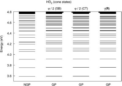
Figure 13. Vibrational levels for the first-excited electronic state of HD2 calculated [8] using: split basis (SB) technique with AðRÞ ¼ j=2; coordinate-transformation (CT) treatment with AðRÞ ¼ j=2; Eq. (A.14) with AðRÞ ¼ gðr; y; jÞ. Shown by the longer line segments are the levels assuming different values in two sets of calculations.

for substantial regions of configuration space where such loops do not encircle the seam, the line integrals yield the value zero for the geometric phase. Such a result may be used to explain why the GP effect has a more remarkable influence on the spectra of H3 than on its isotopic variants [6], as a set of calculations carried out using the split basis technique [6], the coordinatetransformation approach [8], and the GBO equation (A.14) have consistently demonstrated. Note that the first two approaches employed the traditional Longuet-Higgins phase, AðRÞ ¼ j=2, whereas Eq. (A.14) uses a pathdependent phase, AðRÞ ¼ gðr; y; jÞ. The lowest levels calculated by such methods are collected in Figure 13, being the reader addressed to the original papers for details concerning the numerical techniques.

XI. CONCLUDING REMARKS

In this chapter, we discussed the permutational symmetry properties of the total molecular wave function and its various components under the exchange of identical particles. We started by noting that most nuclear dynamics treatments carried out so far neglect the interactions between the nuclear spin and the other nuclear and electronic degrees of freedom in the system Hamiltonian. Due to

such neglect, one must impose the symmetry properties of the nuclear spin in the total wave function. This requires that the total wave function for identical fermions (bosons) must be antisymmetric (symmetric) under the permutation of the identical particles. Kramers’ theorem has been generalized to the case of total angular momentum F. It has then been shown that the states of a system with half-integer total angular momentum quantum number must be degenerate. Because molecular double groups are subgroups of the 3D spatial rotation group SOð3Þ, the former can be used as a powerful means to study the rotational properties of any molecular system. Based on the permutational symmetry requirements of the total wave function and the extented Kramers’ theorem, some severe consequences have then been demonstrated for cases where the nuclear spin quantum number is one-half or zero. The theory has been illustrated by considering in detail the vibrational spectra of the alkali metal trimers where vibronic coupling has been shown to dominate. In this context, we have also reviewed the static and the dynamic Jahn–Teller effects, the GP effect, nonadiabatic coupling, and electron and nuclear spin effects in X3 (2S) systems. Although the discussion on 1H3 and its isotopomers has been brief, it has been pointed out that, for 1H3, the A1 rovibronic states will not be allowed. Thus, for J ¼ 0, only resonant states (hat states) of A2 and E symmetries have physical significance, while only E states are allowed for the pseudobound states (cone states). The implication is that after computing the full spectrum by solving Schrodinger’s equation without consideration of nuclear spin effects, one must carefully distinguish the physically allowed solutions from the unphysical (mathematical) ones. For brevity, no attempt has been made to discuss transition selection rules; the interested reader is referred to [28]. Although the material presented in this chapter focused on Li3 and H3, the theory that has been reviewed, and in some occasions extended, is general and should be of interest to help understand a wider class of systems.

APPENDIX A: GBO APPROXIMATION AND GEOMETRIC PHASE FOR A MODEL TWO-DIMENSIONAL (2D) HILBERT SPACE

Ignoring all nonadiabatic couplings to higher electronic states, the nuclear motion in a two-state electronic manifold is described explicitly in the adiabatic representation by

ðA:2Þ

Then, let the two real electronically adiabatic wave functions be written as [4]

where gðRÞ is the R-dependent mixing angle [5,87–91], which diagonalizes the diabatic potential matrix. By assuming that the electronic basis is orthonormalized, one gets

Now, consider a complex nuclear wave function given by a linear combination of the two real nuclear wave functions [42,53],

After some algebraic manipulation, Eqs. (A.1) and (A.2) lead to the following single-surface equations [4]

ðA:14Þ

which should be valid whenever motion of the nuclei can be confined to the vicinity of the conical intersection, where V1 ’ V2. Note that Eq. (A.14) leads to different sets of eigenvalues depending on whether V1 or V2 are used, except, of course, when V1 ¼ V2, which happens only at the conical intersection. Conversely to Baer and Englmann [25,53], our derivation of Eq. (A.14) has not been based on the assumption (so-called BEB approximation in [92] for the lower sheet equation) that w2 is small enough everywhere, but on the milder premise that w1 and w2 are well behaved. Of course, Eq. (A.14) leads to the corresponding BO equations when the derivative coupling elements are constant or zero.

Now, we discuss how the geometric phase is related to the mixing angle in this two-state model. We begin by writing Eq. (A.11) as the gauge transformation

where w is a real wave function, and AðRÞ is a geometric phase. By analogy, the complex electronic wave function may be written in the form

where ci is the real-valued electronic wave function corresponding to the wave

By using Eq. (A.17), the first derivative coupling for the complex electronic

which shows that, for a set of two electronic states, the derivative coupling is given by the gradient of the geometric phase. A similar result (except for the sign) has been obtained by Baer [25] using a different approach. Note that Eq. (A.20) holds exactly in the vicinity of the crossing seam where the phase AðRÞ is identical for both sheets. From Eqs. (A.4) and (A.20), one then gets

rRAðRÞ ¼ rRgðRÞ ðA:21Þ

which shows that the geometric phase is identical to the mixing angle, except for the sign and a constant term that have no physical implications. Thus, provided that we chose such a constant term to be zero, one has

AðRÞ ¼ gðRÞ ðA:22Þ

Note that the mixing angle has the correct sign-change behavior [5]: gðRÞ ¼ p for a closed path encircling the crossing seam, and gðRÞ ¼ 0 for a closed path that does not encircle it. Thus, the geometric phase defined from Eq. (A.22) displays the correct sign change behavior, while depending on the full set of internal coordinates. Moreover, close to the seam, it shows [5] a behavior similar to the traditional Longuet-Higgins phase of j=2, where j is the pseudorotation angle.

APPENDIX B: ANTILINEAR OPERATORS AND

THEIR PROPERTIES

In this appendix, we review some important properties of antilinear operators

that are used in the text and Appendix C. Let us then consider an operator ^ that

O

well-known example of such an operator. Moreover, as will be shown, the time-

This should apply both to linear and antilinear operators, hereafter denoted,

where ci ði ¼ 1; 2Þ are complex numbers. As for linear operators (where we

are necessary. Note that Eq. (B.1) implies that the norm of a vector cannot be altered both for linear and antilinear operators. More generally, a linear operator cannot change the internal product of two vectors, and hence must be unitary. Conversely, antilinear operators change the internal product to its complex conjugate, and hence are called antiunitary [54]. One has

hcjfi ¼ hfjci ðB:4Þ

which indicates that the unit operator is linear with respect to the ket and antilinear to the bra. In general, a linear operator is linear with respect to the ket and antilinear to the bra. Thus, for an antilinear operator, we have by definition

This implies that the Hermitian conjugate of an antilinear operator is also antilinear. It should also be pointed out that the product of two antilinear