Baer M., Billing G.D. (eds.) - The role of degenerate states in chemistry (Adv.Chem.Phys. special issue, Wiley, 2002)

where we recall that sM, the non-adiabatic coupling matrix, is a real antisymmetric matrix. By multiplying Eq. (B.2) from the right by AM and Eq. (B.1) from the left by AyM and combining the two expressions we get

AyM rAM þ ðrAyMÞAM ¼ ðrAyM AM Þ ¼ 0 ) AyMAM ¼ constant

For a proper choice of boundary conditions, the above mentioned constant matrix can be assumed to be the identity matrix, namely,

Thus AP is a unitary matrix at any point in configuration space.

II.ANALYTICITY

From basic calculus, it is known that a function of a single variable is analytic at a given interval if and only if it has well-defined derivatives, to any order, at any point in that interval. In the same way, a function of several variables is analytic in a region if at any point in this region, in addition to having well-defined derivatives for all variables to any order, the result of the differentiation with respect to any two different variables does not depend on the order of the differentiation.

The fact that the AM matrix fulfills Eq. (B.1) ensures the existence of derivatives to any order for any variable, at a given region in configuration space, if sM is analytic in that region. In what follows, we assume that this is, indeed, the case. Next, we have to find the conditions for a mixed differentiation of the AM matrix elements to be independent of the order.

For that purpose, we consider the p and the q components of Eq. (B.1) (the subscript M will be omitted to simplify notation):

q

qp A þ spA ¼ 0

ðB:4Þ

q qq

By differentiating the first equation according to q we find

Subtracting Eq. (B.11b) from Eq. (B.11a) yields Eq. (B.10), thus proving the existence of Eq. (B.7).

Summary: In a region where the sM elements are analytic functions of the coordinates, AM is an orthogonal matrix with elements that are analytic functions of the coordinates.

APPENDIX C: ON THE SINGLE/MULTIVALUEDNESS OF THE ADIABATIC-TO-DIABATIC TRANSFORMATION MATRIX

In this appendix, we discuss the case where two components of sM , namely, sMp and sMq ( p and q are Cartesian coordinates) are singular in the sense that at least one element in each of them is singular at the point Bð p ¼ a; q ¼ bÞ located on the plane formed by p and q. We shall show that in such a case the adiabatic-to- diabatic transformation matrix may become multivalued.

We consider the integral representation of the two relevant first-order differential equations [namely, the p and the q components of Eq. (19)]:

q

qp AM þ sMpAM ¼ 0

q

ðC:1Þ

qq AM þ sMqAM ¼ 0

In what follows, the subscript M will be omitted to simplify the notations. If the initial point is Pðp0; q0Þ and we are interested in deriving the value of Að AMÞ at a final point Qðp; qÞ then one integral equation to be solved is

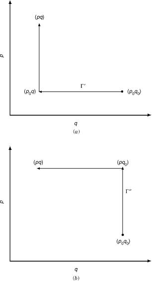
In Eq. (C.2a), we derive the solution by solving it along the path 0

Figure 16. The rectangular paths 0 and 00 connecting the points ( p0; q0) and (p; q) in the (p; q) plane.

and in Eq. (C.2b) by solving it along the path 00 also characterized by two (different) straight lines and the three points (see Fig. 16b)

Note that , formed by 0 and 00 written schematically as

is a closed path.

Since the two solutions of Eq. (C.1) presented in Eqs. (C.2a) and (C.2b) may not be identical we shall derive the sufficient conditions for that to happen.

To start this study, we assume that the four points P, P0, Q0, and Q are at small distances from each other so that if

p ¼ p0 þ p q ¼ q0 þ q

then p and q are small enough distances as required for the derivation. Subtracting Eq. (C.2b) from Eq. (C.2a) yields the following expression:

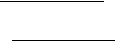
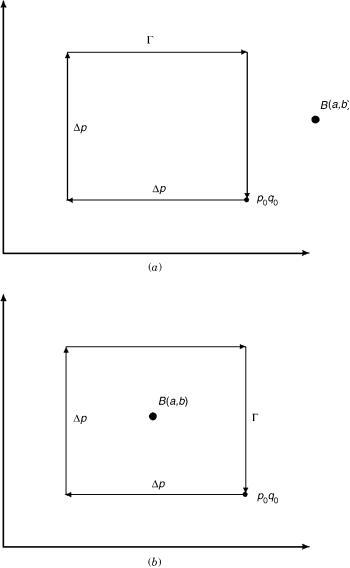
Next, we consider two cases.

1.The case where the point Bða; bÞ is not surrounded by the path (see Fig. 17a). In this case, both sp and sq are analytic functions of the coordinates in the region enclosed by , and therefore the integrands of the two integrals can be replaced by the corresponding derivatives calculated at the respective intermediate points, namely,

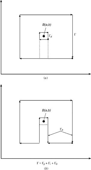
Figure 17. The differential closed paths and the singular point Bða; bÞ in the (p; q) plane: (a) The point B is not surrounded by . (b) The point B is surrounded by .

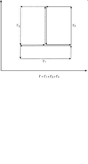
Figure 19 (Continued)

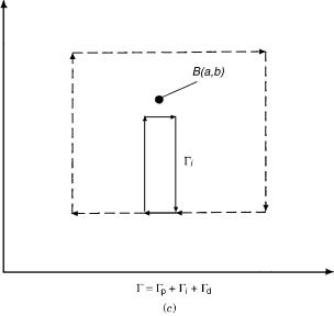
intermediate values cannot be estimated. As a result it is not clear whether the two solutions of the A matrix calculated along the two different differential paths are identical or not. The same applies to a regular size (i.e., not necessarily small) path that surrounds the point Bða; bÞ. This closed path can be constructed from a differential path d that surrounds Bða; bÞ, a path p that does not surround Bða; bÞ, and a third, a connecting path i, which, also, does not surround Bða; bÞ (see Fig. 19). It is noted that the small region surrounded by d governs the features of the A matrix in the entire region surrounded by , immaterial of how large is.

APPENDIX D: THE DIABATIC REPRESENTATION

Our starting equation is Eq. (3) in Section II.A with one difference, namely, we

replace ziðe j nÞ by ziðe j n0Þ; i ¼ 1; . . . ; N, where n0 stands for a fixed set of nuclear coordinates. Thus

XN

Here, ziðe j n0Þ, like ziðe j nÞ, is an eigenfunction of the following Hamiltonian

ðHeðe j n0Þ uiðn0ÞÞziðe j n0Þ ¼ 0 i ¼ 1; . . . ; N ðD:2Þ