Baer M., Billing G.D. (eds.) - The role of degenerate states in chemistry (Adv.Chem.Phys. special issue, Wiley, 2002)

Thus if tjjþ1—the full non-adiabatic coupling term—and the unperturbed non-adiabatic coupling term, t0jjþ1, are assumed to be related to each other as

then it follows, from the above discussion, that the components of the two vectorial perturbations (i.e., dsq jjþ1 and dsyjjþ1) are likely to be (much) smaller than the corresponding components, namely, s0q jjþ1 and s0yjjþ1.

Next, we return to Eq. (25) and recall that we are interested only in the components of sjjþ1 j ¼ 1; 2 in a plane perpendicular to the z axis. It can be shown that if s0jjþ1; j ¼ 1; 2 do not posses a z component, the same applies to the perturbations dsjjþ1 j ¼ 1; 2, as well as to t13.

Substituting Eq. (168) in Eq. (166) and the result in Eq. (25) yields the (inhomogeneous) differential equations for the components of dsjjþ1; j ¼ 1; 2

where the second-order terms were deleted. In this derivation, we employed the fact that:

In the same way, with similar assumptions, we obtain the (inhomogeneous) differential equation for the components of s13

Equation (171) is the an explicit ‘‘curl’’ equation for a coupling that does not has a ‘‘source’’ of its own but is formed due to the interaction between two ‘‘real’’ conical intersection.

Equations (169) and (171), together with Eqs. (170), form the basic equations that enable the calculation of the non-adiabatic coupling matrix. As is noticed, this set of equations creates a hierarchy of approximations starting with the assumption that the cross-products on the right-hand side of Eq. (171) have small values because at any point in configuration space at least one of the multipliers in the product is small [115].

XV. STUDIES OF SPECIFIC SYSTEMS

In this section, we concentrate on a few examples to show the degree of relevance of the theory presented in the previous sections. For this purpose, we analyze the conical intersections of two real two-state systems and one real system resembling a tri-state case.

A.The Study of Real Two-State Molecular Systems

We start by mentioning the studies of Yarkony et al. [64] who were the first to apply the line integral approach to reveal the existence of a conical intersection for a ‘‘real’’ molecular system—the H3 system—by calculating the relevant nonadiabatic coupling terms from first principles and then deriving the topological angle a [see Eq. (76)]. Later Yarkony and co-workers applied this approach to study other tri-atom system such as AlH2 [65], CH2 [66,69], H2S [66], HeH2 [68], and Li3 [70].

Recently, Xu et al. [11] studied in detail the H3 molecule as well as its two isotopic analogues, namely, H2D and D2H, mainly with the aim of testing the ability of the line integral approach to distinguish between the situations when the contour surrounds or does not surround the conical intersection point. Some time later Mebel and co-workers [12,72–74,116] employed ab initio nonadiabatic coupling terms and the line-integral approach to study some features related to the C2H molecule.

Some results of these studies will be presented in Sections XV.A.1–XV.A.3.

1.The H3-System and Its Isotopic Analogues

Although the study to be described is for a ‘‘real’’ system, the starting point was not the ab initio adiabatic potential energy surfaces and the ab initio nonadiabatic coupling terms but a diabatic potential [117], which has its origin in the LSTH potential [118] improved by including three-center terms [119]. These were used to calculate the adiabatic-to-diabatic transformation angle g by employing the Hellmann–Feynman theorem [3,36]. However, we present our results in term of the diabatic-to-adiabatic transformation angle b, which is also know as the mixing angle. We start by proving, analytically that these two angles are identical up to an integration constant.

We consider a 2D diabatic framework that is characterized by an angle, bðsÞ, associated with the orthogonal transformation that diagonalizes the diabatic potential matrix. Thus, if V is the diabatic potential matrix and if u is the adiabatic one, the two are related by the orthogonal transformation matrix A [34]:

where Ay is the complex conjugate of the A matrix. For the present two-state case, A can be written in the form:

where b—the above mentioned mixing angle—is given by [36a]:

Recalling g(s), the adiabatic-to-diabatic transformation angle [see Eqs. (74) and (75)] it is expected that the two angles are related. The connection is formed by the Hellmann–Feynman theorem, which yields the relation between the s component of the non-adiabatic coupling term, s, namely, ss, and the characteristic diabatic magnitudes [13]

where Ai, i ¼ 1; 2 are the two columns of the A matrix in Eq. (173). By replacing the two Ai columns by their explicit expressions yields for ts the expression

and by substituting Eq. (177) in Eq. (176), yields the following result for ssðsÞ:

Comparing this equation with Eq. (75), it is seen that the mixing angle b is, up to an additive constant, identical to the relevant adiabatic-to-diabatic transforma- tion—angle g:

This relation will be used to study geometrical phase effects within the diabatic framework for the H3 system and its two isotopic analogues. What is meant by

this is that since our starting point is the 2 2 diabatic potential matrix, we do not need to obtain the adiabatic-to-diabatic transformation angle by solving a line integral; it will be obtained simply by applying Eqs. (174) and (178). The forthcoming study is carried out by presenting bðjÞ as a function of an angle j to be introduced next.

In the present study, we are interested in finding the locus of the seam defined by the conditions rAB ¼ rBC ¼ rAC [14–17] where rAB, rBC, and rAC are the interatomic distances. Since we intend to study the geometrical properties produced by this seam we follow a suggestion by Kuppermann and co-workers [29,120,121] and employ the hyperspherical coordinates (r; y; j) that were found to be suitable for studying topological effects for the H H2 (and its isotopic analogues) because one of the hyperspherical (angular) coordinates surrounds the seam in case of the pure-hydrogenic case. Consequently, following previous studies [29,122–124], we express the three above-mentioned distances in terms of these coordinates, that is,

By equating the three interatomic distances with each other, we find that the seam is a straight line, for which r is arbitrary but j and y have fixed values js and ys determined by the masses only.

Equations (182)–(185) are valid when all three masses are different. In case two masses are equal, namely, mB ¼ mC, we get for ys the simplified expression

all three masses are equal (then t ¼ 1), we get ys ¼ 0 and js ¼ p.

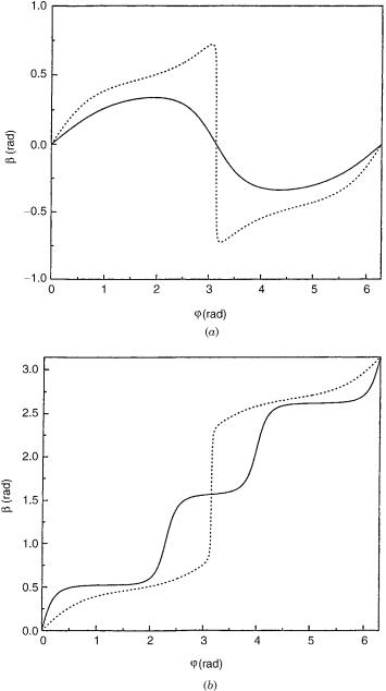
In what follows, we discuss the H2D system. For this purpose Eq. (186) is employed for which it is obtained that the straight line seam is defined for the following values of ys and js, namely, ys ¼ 0:4023 rad, and js ¼ p. In the H3 case, the value of ys is zero and this guarantees that all the circles with constant r and y encircle the seam. The fact that ys is no longer zero implies that not all the circles with constant r and y encircle the seam; thus, circles for which y > ys will encircle the seam and those with y < ys will not.

In Figure 10 are presented bðjÞ curves for H2D, all calculated for r ¼ 6a0. In this calculation, the hyperspherical angle j, defined in along the [0;2p] interval, is the independent angular variable. Figure 10a shows two curves for the case where the line integral does not encircle the seam, namely, for y ¼ 0:2 and 0.4 rad and in Figure 10b for the case where the line integral encircles the seam, namely, for y ¼ 0:405 and 2.0 rad. Notice that the curves in Figure 10a reach the value of zero and those in Figure 10b reach the value of p. In particular, two curves, that in Figure 10a for y ¼ 0:4 rad and the other in Figure 10b for y ¼ 0:405 rad, were calculated along very close contours (that approach the locus of the seam) and indeed their shapes are similar—they both yield an abrupt step—but one curve reaches the value of zero and the other the value p. Both types of results justify the use of the line integral to uncover the locus of the seam. More detailed results as well as the proper analysis can be found in [11].

These results as well as others presented in [11] are important because on various occasions it was implied that the line integral approach is suitable only

for cases when relatively small radii around the conical intersection are applied [64]. In [11], it is shown for the first time that this approach can be useful even for large radii, which does not mean that it is relevant for any assumed contour surrounding a conical intersection (or for that matter a group of conical intersections) but means that we can always find contours with large radii that will reveal the conical intersection location for a given pair of states.

2.The C2H-Molecule: The Study of the (1,2) and the

(2,3) Conical Intersections

In the first part of this study, we were interested in non-adiabatic coupling terms between the 12A0 and 22A0 and between the 22A0 and 32A0 electronic states. The calculations were done employing MOLPRO [6], which yield the six relevant non-adiabatic coupling elements as calculated with respect to the Cartesian center-of-mass coordinates of each atom. These coupling terms were then transformed, employing chain rules [12,73], to non-adiabatic coupling elements with respect to the internal coordinates of the C2H molecule, namely, hzijqzj=qr1i

ð¼ tr1 Þ; hzijqzj=qr2ið¼ tr2 Þ, and hzijqzj=qjið¼ tjÞ. Here r1 and r2 are the C C and C H distances, respectively, and j is the relevant CC CH angle. The

adiabatic-to-diabatic transformation angle, gðjjr1; r2Þ, is derived next employing the following line integral [see Eq. (75)], where the contour is an arc of a circle with radius r2:

The corresponding topological phase, aðr1; r2Þ [see Eq. (76)] defined as gðj ¼ 2p j r1; r2Þ, was also obtained for various values of r1 and r2.

First, we refer to the (1,2) conical intersection. A detailed inspection of the

non-adiabatic coupling terms revealed the existence of a conical intersection

fj ¼ ¼ ˚ between these two states, for example, at the point 0 r1 1 35 A,

; :

¼ ˚ Þ

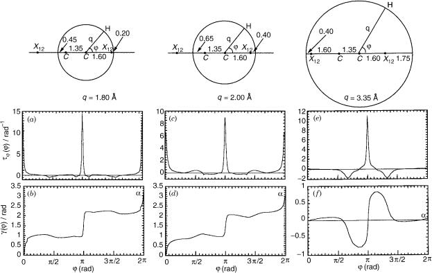
r2 1:60 A as was established before [105]. More conical intersections of this kind are expected at other r1 values. Next, were calculated the gðj j r1; r2Þ angles as a function of j for various r2. The tjðj j r1; r2Þ functions as well as the adiabatic-to-diabatic transformation angles are presented in Figure 11 for

¼ ˚

three different r2 values, namely, r2 1:8; 2:0; 3:35 A. Mebel et al. [12] also calculated the topological angle aðr1; r2Þ for these three r2 values employing Eq. (76) and got, for the first two r2 values, the values 3.136 and 3.027 rad, respectively—thus, in both cases, values close to the expected p value. A different situation is encountered in the third case when the circle surrounds the two (symmetrical) CIs as can be seen from the results presented in the third panel of Figure 11e and f. In such a case, the angle a is expected to be either an even multiple of p or zero. The integration according to Eq. (76) yields the value

of 0.048 rad, namely, a value close to zero. It is important to mention that we also performed integrations along closed circles that do not surround any conical intersections and got the value zero as was proved in Appendix C (for more details about these calculations see [12]).

In this series of results, we encounter a somewhat unexpected result, namely, when the circle surrounds two conical intersections the value of the line integral is zero. This does not contradict any statements made regarding the general theory (which asserts that in such a case the value of the line integral is either a multiple of 2p or zero) but it is still somewhat unexpected, because it implies that the two conical intersections behave like vectors and that they arrange themselves in such a way as to reduce the effect of the non-adiabatic coupling terms. This result has important consequences regarding the cases where a pair of electronic states are coupled by more than one conical intersection.

On this occasion, we want also to refer to an incorrect statement that we made more than once [72], namely, that the (1,2) conical intersection results indicate ‘‘that for any value of r1 and r2 the two states under consideration form an isolated two-state sub-Hilbert space.’’ We now know that in fact they do not form an isolated system because the second state is coupled to the third state via a conical intersection as will be discussed next. Still, the fact that the series of topological angles, as calculated for the various values of r1 and r2, are either multiples of p or zero indicates that we can form, for this adiabatic two-state system, single-valued diabatic potentials. Thus if for some numerical treatment only the two lowest adiabatic states are required, the results obtained here suggest that it is possible to form from these two adiabatic surfaces singlevalued diabatic potentials employing the line-integral approach. Indeed, recently Billing et al. [104] carried out such a photodissociation study based on the two lowest adiabatic states as obtained from ab initio calculations. The complete justification for such a study was presented in Section XI.

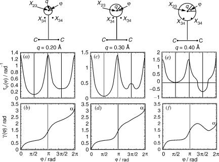
Reference [73] presents the first line-integral study between two excited states, namely, between the second and the third states in this series of states. Here, like before, the calculations are done for a fixed value of r1 (results are reported for r1 ¼ 1:251 A˚) but in contrast to the previous study the origin of the system of coordinates is located at the point of this particular conical intersection, that is, the (2,3) conical intersection. Accordingly, the two polar coordinates (j; q) are defined. Next is derived the j-th non-adiabatic coupling term i.e. tj ð¼ hz2jqz3=qjiÞ again employing chain rules for the transformation ðtg; tr2Þ ! tj(tq is not required because the integrals are performed along a

tjðj j qÞ exhibits the following symmetry properties: tjðjÞ ¼ tjðp jÞ and

Figure 12. Results for the C2H molecule as calculated along a circle surrounding the 22A0–32A0

˚

conical intersection. The conical intersection is located on the C2v line at a distance of 1.813 A from

¼ ˚

the CC axis, where r1 ( CC distance) 1.2515 A. The center of the circle is located at the point of the conical intersection and defined in terms of a radius q. Shown are the non-adiabatic coupling matrix elements tjðjjqÞ and the adiabatic-to-diabatic transformation angles gðjjqÞ as calculated for

tjðp þ jÞ ¼ tjð2p jÞ, where 0 j p. In fact, since the origin is located on the C2v axis we should expect only jtjðjÞj ¼ jtjðp jÞj and jtjðp þ jÞj ¼ jtjð2p jÞj, where 0 j p but due to continuity requirements these relations also have to be satisfied without the absolute signs. (2) It is seen that the adiabatic-to-diabatic transformation angle, gðj j qÞ, increases, for the two smaller q-values, monotonically to become að j qÞ, with the value of p (in

p p ¼ ˚

fact, we got 0.986 and 1.001 for q 0:2 and 0.3 A, respectively). The two-

¼ ˚

state assumption seems to break down in case q 0:4 A because the calculated value of að j qÞ is not anymore p but only 0.63p. The reason being that the

¼ ˚

q 0:4-A circle not only passes too close to two (3,4) conical intersections—

˚

the distances at the closest points are 0.04 A—and so the (2,3) system can not be considered anymore as an isolated sub-Hilbert space but in fact surrounds these two conical intersections (see third panel of Fig. 12). More details are given in Section XV.B [116].