Baer M., Billing G.D. (eds.) - The role of degenerate states in chemistry (Adv.Chem.Phys. special issue, Wiley, 2002)

configuration space but have to be further developed, if several conical intersections are located at the region of interest.

Now we intend to present the purpose of this section. In order to do this in a comprehensive way, we need to explain what is meant, within the present framework, by the statement that ‘‘the diabatization is non-physical.’’ The procedure discussed above is based on a transformation matrix of a dimension M derived within a sub-Hilbert space of the same dimension. The statement ‘‘a diabatization is non-physical’’ implies that some of the elements of the diabatic matrix formed in this process are multivalued in configuration space. (In this respect, it is important to emphasize that the nuclear Schro¨dinger equation cannot be solved for multivalued potentials.) We show that if an M-dimensional sub-Hilbert space is not large enough, some elements of the diabatic potential matrix will not be single valued. Thus a resolution to this difficulty seems to be in increasing the dimension of the sub-Hilbert space, that is, the value of M. However, increasing M indefinitely will significantly increase the computational volume. Therefore it is to everyone’s interest to keep M as small as possible. Following this explanation, we can now state the purpose of this section:

We intend to show that an adiabatic-to-diabatic transformation matrix based on the non-adiabatic coupling matrix can be used not only for reaching the diabatic framework but also as a mean to determine the minimum size of a sub-Hilbert space, namely, the minimal M value that still guarantees a valid diabatization.

For example: one forms, within a two-dimensional (2D) sub-Hilbert space, a 2 2 diabatic potential matrix, which is not single valued. This implies that the 2D transformation matrix yields an invalid diabatization and therefore the required dimension of the transformation matrix has to be at least three. The same applies to the size of the sub-Hilbert space, which also has to be at least three. In this section, we intend to discuss this type of problems. It also leads us to term the conditions for reaching the minimal relevant sub-Hilbert space as ‘‘the necessary conditions for diabatization.’’

In this section, diabatization is formed employing the adiabatic-to-diabatic transformation matrix A, which is a solution of Eq. (19). Once A is calculated, the diabatic potential matrix W is obtained from Eq. (22). Thus Eqs. (19) and (22) form the basis for the procedure to obtain the diabatic potential matrix elements.

Note that since the adiabatic potentials are single valued by definition, the single valuedness of W (viz, the single valuedness of each of its terms) depends on the features of the A matrix [see Eq. (22)]. It is also obvious that if A is single valued, the same applies to W [the single valuedness of the A matrix in a given region is guaranteed if Eq. (25) is fulfilled throughout this region]. However, in Section (IV.A) we showed that A does not have to be single valued in order to guarantee the single valuedness of W. In fact, it was proved that the necessary condition for having single-valued diabatic potentials along a given

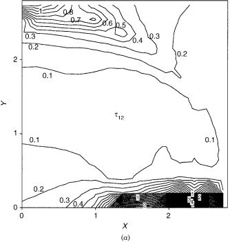
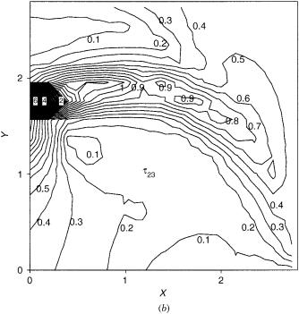
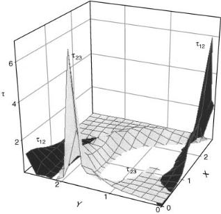
Figure 7. The geometrical positions (with respect to the CC axis) of s12ðx; yÞ and s23ðx; yÞ. All

˚ y

distances are in angstroms (A). The Cartesian coordinates (x; y) are related to (q; ) as follows: x ¼ q cos y; y ¼ q sin y, where q and y are measured with respect to the midpoint between the two carbons.

to Section VI, for this purpose we need the three states because the two lowest states (1 and 2) and the two highest states (2 and 3) are strongly coupled to each other. Next, we examine to see if under these conditions this is really necessary or could the diabatization be achieved with only the two lowest states.

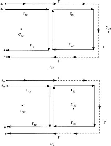
For this purpose, we consider Figure 8 with the intention of examining what happens along the contour , in particularly when it gets close to C23. Note that some segments of the contour are drawn as full lines and others are as dashed lines. The full lines denote segments along which s12ðsÞ is of a strong intensity but s23ðsÞ is negligibly weak. The dashed lines denote segments along which s12ðsÞ is negligibly weak.

Next, consider the following line integral [see Eq. (27)]:

Figure 8. The representation of an open contour in terms of an open contour 12 in the vicinity of the conical intersection at C12 and a closed contour 23 at the vicinity of a conical intersection at C23: ¼ 12 þ 23. It is assumed that the intensity of s12 is strong along 12 (full line) and weak along 23 (dashed line). (a) The situation when C23 is outside the closed contour 23. (b) The situation when C23 is inside the closed contour 23.

where AðsÞ and sðsÞ are of dimensions 3 3 [the explicit form of sðsÞ is given in Eq. (99)]. We also consider the two other s matrices, namely, s12ðsÞ and s23ðsÞ (see Eq. (105)] and it is easy to see that

To summarize: Following the theory presented above, we have to distinguish between two situations. (1) As long as does not surround C23 the matrix AðsÞ

(2) In the case where surrounds the C23 conical intersection, the value of g12ðsÞ may change its sign (for more details see Ref. [108]).

Since for any assumed contour the most that can happen, due to C23, is that g12ðsÞ flips its sign, the corresponding 2 2 diabatic matrix potential, WðsÞ, will not be affected by that as can be seen from the following expressions:

In other words, the calculation of W can be carried out by ignoring C23 [or s23ðsÞ] altogether.

XII. THE ADIABATIC-TO-DIABATIC TRANSFORMATION MATRIX AND THE WIGNER ROTATION MATRIX

The adiabatic-to-diabatic transformation matrix in the way it is presented in Eq. (28) is somewhat reminiscent of the Wigner rotation matrix [109a] (assuming that Aðs0Þ IÞ. In order to see this, we first present a few well-known facts related to the definition of ordinary angular momentum operators (we follow the presentation by Rose [109b] and the corresponding Wigner matrices and then return to discuss the similarities between Wigner’s djðbÞ matrix and the adiabatic-to-diabatic transformation matrix.

A.Wigner Rotation Matrices

The ordinary angular rotation operator R(k,y) in the limit y ! 0 is written as

where k is a unit vector in the direction of the axis of rotation, y is the angle of rotation, and S(k,y) is an operator that has to fulfill the condition Sðk; yÞ ! 0 for y ! 0 to guarantee that in this situation (i.e., when y ! 0) Rðk; yÞ ! I. Moreover, since Rðk; yÞ has to be unitary, the operator Sðk; yÞ has to be Hermitian. Next, it is shown that Sðk; yÞ is related to the total angular momentum operator, J, in the following way:

where the dot stands for scalar product. By substituting Eq. (127) in Eq. (126) we get the following expression for Rðk; yÞ:

It has to be emphasized that in this framework J is the angular momentum operator in ordinary coordinate space (i.e., configuration space) and y is a (differential) ordinary angular polar coordinate.

Next, Euler’s angles are employed for deriving the outcome of a general rotation of a system of coordinates [86]. It can be shown that Rðk; yÞ is accordingly presented as

where Jy and Jz are the y and the z components of J and a, b, and g are the corresponding three Euler angles. The explicit matrix elements of the rotation operator are given in the form:

where m and m0 are the components of J along the Jz and Jz0 axes, respectively, and jjmi is an eigenfunction of the Hamiltonian of J2 and of Jz. Equation (130) will be written as

The Dj matrix as well as the d j matrix are called the Wigner matrices and are the subject of this section. Note that if we are interested in finding a relation between the adiabatic-to-diabatic transformation matrix and Wigner’s matrices, we should mainly concentrate on the d j matrix. Wigner derived a formula for

these matrix elements [see [109b], Eq. (4.13)] and this formula was used by us to obtain the explicit expression for j ¼ 32 (the matrix elements for j ¼ 1 are given in [109b], p. 72).

B.The Adiabatic-to-Diabatic Transformation Matrix and

the Wigner dj Matrix

The obvious way to form a similarity between the Wigner rotation matrix and the adiabatic-to-diabatic transformation matrix defined in Eqs. (28) is to consider the (unbreakable) multidegeneracy case that is based, just like Wigner rotation matrix, on a single axis of rotation. For this sake, we consider the particular set of s matrices as defined in Eq. (51) and derive the relevant adiabatic-to- diabatic transformation matrices. In what follows, the degree of similarity between the two types of matrices will be presented for three special cases, namely, the two-state case which in Wigner’s notation is the case, j ¼ 12, the tri-state case (i.e., j ¼ 1) and the tetra-state case (i.e., j ¼ 32).

However, before going into a detail comparison between the two types of matrices it is important to remind the reader what the elements of the Jy matrix look like. By employing Eqs (2.18) and (2.28) of [109b] it can be shown that

It is expected that for a certain choice of parameters (that define the s matrix) the adiabatic-to-diabatic transformation matrix becomes identical to the corresponding Wigner rotation matrix. To see the connection, we substitute Eq. (51) in Eq. (28) and assume Aðs0Þ to be the unity matrix.

The three matrices of interest were already derived and presented in Section V.A. There they were termed the D (topological) matrices (not related to the above mentioned Wigner Dj matrix) and were used to show the kind of quantization one should expect for the relevant non-adiabatic coupling terms. The only difference between these topological matrices and the