Baer M., Billing G.D. (eds.) - The role of degenerate states in chemistry (Adv.Chem.Phys. special issue, Wiley, 2002)

the non-adiabatic coupling terms and to connect them with pseudomagnetic fields.

A.The Non-Adiabatic Coupling term as a Vector Potential

In Section III.B, and later in Appendix C, it was shown that the sufficient condition for the adiabatic-to-diabatic transformation matrix A to be single valued in a given region in configuration space is the fulfillment of the following ‘‘curl’’ condition [8,34]:

This condition is fulfilled as long as the components of t are analytic functions at the point under consideration (in case part of them become singular at this point, curl t is not defined).

The expression in Eq. (137) is reminiscent of the Yang–Mills field, however, it is important to emphasize that the Yang–Mills field was introduced for a different physical situation [58,59]. In fact, what Eq. (137) implies is that for molecular systems the Yang–Mills field is zero if the following two conditions are fulfilled:

1.The group of states, for which Eq. (137) is expected to be valid, forms a sub-Hilbert space that is isolated with respect to other portions of the Hilbert space following the definition in Eqs. (40).

2.The s-matrix elements are analytic functions (vectors) in the abovementioned region of configuration space.

In what follows, we assume that indeed the group of states form an isolated sub-Hilbert space, and therefore have a Yang–Mills field that is zero or not will depend on whether or not the various elements of the s matrix are singular.

In order to extend the existence of Eq. (137) for the singular points as well we write it as follows:

where H is zero at the regular points.

In order to get more insight, we return to the Born–Oppenheimer–Huang equation [1,2] as written in Eq. (16) and, for simplicity, limit ourselves to the two-state case:

so that s is given in the form

Although Eq. (139) looks like a Schro¨dinger equation that contains a vector potential s, it cannot be interpreted as such because s is an antisymmetric matrix (thus, having diagonal terms that are equal to zero). This ‘‘inconvenience’’ can be ‘‘repaired’’ by employing the following unitary transformation:

where t is now a diagonal matrix

and w is an ordinary potential matrix of the kind

The important outcome from this transformation is that now the nonadiabatic coupling term s is incorporated in the Schro¨dinger equation in the same way as a vector potential due to an external magnetic field. In other words, s behaves like a vector potential and therefore is expected to fulfill an equation of the kind [111a]

where H is a pseudomagnetic field. Equation (146) looks similar to Eq. (138) but is in fact identical to it because in the case of two states the cross-term ½s s& is zero. Now, by returning to the Yang–Mills field we recall that H 6¼ 0 at the singular points of s. In the present study, we consider a case of one singular point.

The question is if in reality such magnetic fields exist. It turns out that such fields can be formed by long and narrow solenoids [111b]. It is well known that in this case the magnetic fields are nonzero only inside the solenoid but zero

outside it [111b]. Moreover, it has a nonzero component along the solenoid axis only. Thus simulating the molecular seam [36,54,110] as a solenoid we can identify the non-adiabatic coupling term as a vector potential produced by an infinitesimal narrow solenoid.

The quantum mechanical importance of a vector potential A, in regions where the magnetic field is zero, was first recognized by Aharonov and Bohm in their seminal 1959 paper [112].

B.The Pseudomagnetic Field and the Curl Equation

To continue, we assume the following situation: We concentrate on an x–y plane, which is chosen to be perpendicular to the seam. In this way, the pseudomagnetic field is guaranteed to be perpendicular to the plane and will have a nonzero component in the z direction only. In addition, we locate the origin at the point of the singularity, that is, at the crossing point between the plane and the seam. With these definitions the pseudomagnetic field is assumed to be of the form [113].

Here, dðqÞ is the Dirac d function and f ðyÞ is an arbitrary function to be determined [it can be shown that any function of the type f ðq; yÞ leads to the same result because of the dðqÞ function]. By considering Eq. (146) for the z component, we obtain (employing polar coordinates):

Here, (tq; ty) are the radial and the angular components of s (the z component, i.e., the out-of-plane component, is by definition equal to zero). Equation (148) can be shown (by substitution) to have the following solution:

tyðq; yÞ ðq dq qtq ¼ phðqÞ f ðyÞ ð149Þ

0 qy

Since q is a radius it is always positive, and therefore Eq. (149) can be written, without loss of generality, as

Next, we consider the ‘‘quantization’’ condition introduced earlier [see Eq. (94)]. Assuming to be a circle with radius q, Eq. (94) implies

ð2p

0

A similar integration over y along the (0,2p) range can be carried out for Eq. (151). Thus, let us first consider the integration over the second term

In Section XIV.A, it is proved that tqðq; yÞ is, for every value of q, single valued with respect to y so that we have

Combining Eqs. (151)–(153) yields the following outcome:

ð2p

0

In other words, the quantization that was encountered for the non-adiabatic coupling terms is associated with the ‘‘quantization’’ of the intensity of the ‘‘magnetic’’ field along the seam. Moreover, Eq. (154) reveals another feature, namely, that there are fields for which n is an odd integer, namely, conical intersections and there are fields for which n is an even integer, namely, parabolical intersections.

Equation (151) can be applied to obtain f ðyÞ. Ab initio calculation for small enough q values will yield tyðy; q 0Þ and these, as is seen from Eq. (151), can be directly related to f ðyÞ:

where the contribution of the second term on the left-hand side (for small enough q values) is ignored.

C.Conclusions

This section is devoted to the idea that the electronic non-adiabatic coupling terms can be simulated as vector potentials. For this purpose, we considered

a two-state system, shifted (rigorously) the off-diagonal non-adiabatic coupling terms to the diagonal and employed the relevant Maxwell equation. As is also noticed, the simulation created a connection between the ‘‘curl’’ condition as fulfilled by the non-adiabatic coupling terms and the Yang–Mills field.

As noticed, a pseudomagnetic field is assumed to exist along the seam formed by varying indirect coordinates (i.e., coordinates not related to the plane for which the vector potential is not zero) of a given molecular system. In this respect, we want to suggest that eventually the pseudomagnetic field is ‘‘formed,’’ semiclassically, by the zero-point vibrational motion of the indirect coordinates. For this purpose, we consider a three-atom molecular system ABC and assume the AB distance to be the indirect coordinate. Varying the AB distance builds up, semiclassically, a motion along the seam. Consequently, the zero-point vibrational motion along the AB bond creates, semiclassically, a periodic motion along the seam. This motion eventually causes charges that are concentrated along the seam (or its vicinity) to oscillate and in this way to form a pseudoelectromagnetic field.

XIV. A THEORETIC-NUMERIC APPROACH TO CALCULATE THE ELECTRONIC NON-ADIABATIC COUPLING TERMS

In this section, we discuss the possibility that the electronic non-adiabatic coupling terms will be derived, not by ab initio treatments but, by solving the curl equations for a given set of boundary conditions obtained from ab initio calculations [114,115]. In other words, instead of performing an ab initio calculation at any point in configuration space we suggest solving the relevant differential equations for boundary conditions obtained from a (limited) ab initio calculation [64–74] or perturbation theory [66,67].

A.The Treatment of the Two-State System in a Plane

1.The Solution for a Single Conical Intersection

The curl equation for a two-state system is given in Eq. (26):

Equation (26) is fulfilled at any point in configuration space for which the components of s are analytic functions.

Equation (26) is a set of partial first-order differential equations. Each component of the Curl forms an equation and this equation may or may not be ‘‘coupled’’ to the other equations. In general, the number of equations is equal to the number of components of the Curl equations. At this stage, to solve this set of equation in its most general case seems to be a formidable task.

This result implies that sqðq; yÞ is, for every value of q, single valued with respect to y.

In what follows, we assume that the second term in Eq. (158a) is negligibly small and as a result syðq; yÞ becomes independent of q. Thus

where q0 is a fixed q value and syðq ¼ q0; yÞ is a boundary value (at q0 0) for syðq; yÞ determined either by ab initio calculations or perturbation theory. We also recall that syðq; yÞ fulfills the quantization condition as written in Eq. (159).

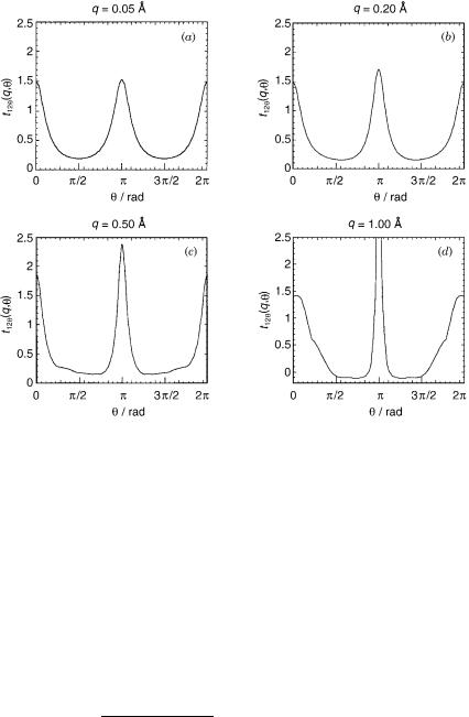
To examine our assumption regarding the dependence of syðq; yÞ on q, we consider the well-known (collinear) conical intersection of the C2H molecule formed by the two lowest states, namely, the 12A0 and the 22A0 states [12,72,105]. Figure 9 presents syðq; yÞ as calculated for a fixed C C distance,

¼ ˚

that is, RCC 1:35 A and for different q values. It is seen that the basic shape of

syðq; yÞ is approximately preserved although q is varied along a relative large

˚ s ð yÞ interval, that is, the [0.05, 1.0 A] interval. It is noticed that the shape y q is

;

¼ ˚ y p

significantly affected only when q 1 A and . The reason is that in this

ð ¼ ˚ y ¼ pÞ

situation the point q 1 A; gets very close to one of the carbons (the

˚ s ð yÞ distance becomes 0.3 A) and therefore the ab initio values for y q; are not

for an isolated conical intersection anymore as it should be [12].

In Section XIV.A.2, we intend to obtain the vector function sðq; yÞ for a given distribution of conical intersections. Thus, first we have to derive an expression for a conical intersection removed from the origin, namely, assumed to be located at some point, (qj0; yj0), in the plane.

Combining Eqs. (151), (158a), and (161a) we get that syðq; yÞ can be writtern

To shift it to some arbirtrary point (qj0; yj0) we first express Eq. (161b) in terms of Cartesian coordinates, and then shift the solution to the point of interest, namely, to ðxj0; yj0Þ½ ðqj0; yj0Þ&. Once completed, the solution is transformed back to polar coordinates (for details see Appendix F). Following

this procedure, syðq; yÞ and sqðq; yÞ (which is now different from zero) become

where qj and yj are the coordinates of an arbitrary point, Pðq; yÞ, with respect to the conical intersection position. The coordinates (qj; yj) are related to ðq;yÞ as

In Eq. (162) [as well as in Eq. (164)], we attached a subscript j to f ðyÞ to indicate that each conical intersection (in this case the jth one) may form a different spatial (angular) distribution.

Note that for qj0 ¼ 0 the solution in Eq. (161b) is restored (and sq becomes zero).

2.The Solution for a Distribution of Conical Intersections

With the modified expression we can now extend the solution of Eq. (162) to any number of conical intersections. The solution in Eq. (162) stands for a single conical intersection located at an arbitrary point (qj0; yj0). Since syðq; yÞ and sqðq; yÞ are scalars the solution in case of N conical intersections located at the

Equation (165) yields the two components of sðq; yÞ, the vectorial nonadiabatic coupling term, for a distribution of two-state conical intersections expressed in terms of the values of the angular component of each individual non-adiabatic coupling term at the closest vicinity of each conical intersection. These values have to be obtained from ab initio treatments (or from perturbation expansions); however, all that is needed is a set of these values along a single closed circle, each surrounding one conical intersection.

To summarize our findings so far, we may say that if indeed the radial component of a single completely isolated conical intersection can be assumed to be negligible small as compared to the angular component, then we can present, almost fully analytically, the 2D ‘‘field’’ of the non-adiabatic coupling terms for a two-state system formed by any number of conical intersections. Thus, Eq. (165) can be considered as the non-adiabatic coupling field in the case of two states.

In Section XIV.B, this derivation is extended to a three-state system.

B.The Treatment of the Three-State System in a Plane

To study the three-state case, we consider two non-adiabatic coupling terms: one, between the lowest and the intermediate state, designated as t12 with its origin located at Paðqa; yaÞ, and the other between the intermediate and the highest state, designated as t23 with its origin located at Pbðqb; ybÞ. As will be seen, in addition to t12 and t23 we also have to consider t13, although no degeneracy point

exists between the lowest and the highest states. In other words, we shall show how the interaction between the above mentioned two conical intersections builds up t13, which does not have a source of its own. Thus the s matrix for the most general case has to be of the form:

01

The curl equation for three (or more) states is given in Eq. (25) and is presented here again for the sake of completeness:

Eq. (25) contains an additional, nonlinear term. This nonlinear term enforces a perturbative scheme in order to solve the required s-matrix elements.

The derivation of the s-matrix elements will be done in two steps: (1) first by considering each of the conical intersection as being isolated, namely, the one independent of the other; and (2) secondly by employing Eq. (20) to treat the two conical intersections as one complete system. Thus within the first step we obtain zeroth-order expressions for s12 and s23, that is, s012 and s023, respectively, whereas within the second step we not only correct these expressions so that Eq. (25), is ( ) fulfilled for three states, but also derive the missing s13 term. The study is done, as before, for a plane in configuration space employing polar coordinates.

To study the two isolated conical intersections, we have to treat two-state curl equations that are given in Eq. (26). Here, the first 2 2 s matrix contains the (vectorial) element, that is, s012 and the second 2 2 s matrix contains s023. As before each of the non-adiabatic coupling terms, s012 and s023 has the following components:

s0jjþ1 ¼ ðs0q jjþ1; s0yjjþ1Þ j ¼ 1; 2 ð167Þ

where s0qjjþ1 and s0yjjþ1; j ¼ 1, 2, were derived in Section XIV.A [see Eqs. (165)], and therefore no further treatment is necessary.

In Section XI.B, we discussed situations (based on ab initio calculations) where the two non-adiabatic coupling terms t12 and t23 slightly overlap [12,108]. Based on ab initio calculations (as were carried out for the C2H molecule) it was found that in many cases the non-adiabatic coupling is not evenly distributed around its point of degeneracy but rather is concentrated along a radial ridge that starts at the point of degeneracy (see Figs. 6 and 7). Therefore, in these cases, only slight overlaps are expected, in particular, when the two points of degeneracy Pxðqx; yxÞ; x ¼ a; b are located far enough from each other [108].