Baer M., Billing G.D. (eds.) - The role of degenerate states in chemistry (Adv.Chem.Phys. special issue, Wiley, 2002)

The case of M ¼ 3 is somewhat more complicated because the corresponding orthogonal matrix is expressed in terms of three angles, namely, g12, g13, and g23 [36,84,85]. This case was recently studied by us in detail [85] and here we briefly repeat the main points.

The matrix Að3Þ is presented as a product of three rotation matrices of the form:

[the other two, namely, Qð123Þðg12Þ and Qð233Þðg23Þ, are of a similar structure with the respective cosine and sine functions in the appropriate positions) so that Að3Þ becomes:

Here, cij ¼ cosðgijÞ and sij ¼ sinðgijÞ. The three angles are obtained by solving the following three coupled first-order differential equations, which follow from Eq. (19) [36,84,85]:

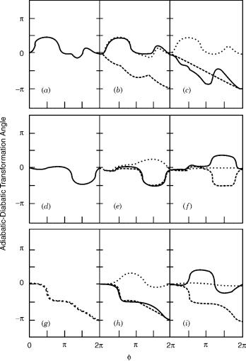
These equations were integrated as a function of j (where 0 j 2pÞ, for a model potential [85] along a circular contour of radius r (for details see Appendix E). The j-dependent g angles, that is, gijðj j rÞ, for various values of r and e ( e is the potential energy shift defined as the shift between the two original coupled adiabatic states and a third state, at the origin, i.e., at r ¼ 0:Þ are presented in Figure 1. Thus for each j we get, employing Eq. (81), the Að3ÞðjÞ matrix elements. The relevant Dð3Þ matrix is obtained from Að3Þ by substituting j ¼ 2p. If aij are defined as

then, as is noticed from Figure 1, the values of aij are either zero or p. A simple analysis of Eq. (81), for these values of aij, shows that Dð3Þ is a diagonal matrix with two ( 1) terms and one (þ1) in the diagonal.

Figure 1. The three adiabatic–diabatic transformation angles [obtained by solving Eqs. (77) for a 3 3 diabatic model potential presented in Section XIII.B] g12ðjÞ, g23ðjÞ, g13ðjÞ as calculated

for different values of rand e: (a) g ¼ g12, e ¼ 0:0; (b) g ¼ g12, e ¼ 0:05; (c) g ¼ g12, e ¼ 0:25; (d) g ¼ g23, e ¼ 0:0; (e) g ¼ g23, e ¼ 0:05; ( f ) g ¼ g23, e ¼ 0:25; (g) g ¼ g13, e ¼ 0:0; (h) g ¼ g13, e ¼ 0:05; (i) g ¼ g13, e ¼ 0:25. ———— r ¼ 0:01; - - - - - - - r ¼ 0:1; ..............

r ¼ 0:5.

This result will now be generalized for an arbitrary Dð3Þ matrix in the following way: Since a general Að3Þ matrix can always be written as in Eq. (81) the corresponding Dð3Þ matrix becomes diagonal if and only if:

This expression shows that the Dð3Þ matrix, in the most general case, can have either three (þ1) terms in the diagonal or two ( 1) terms and one (þ1). In the first case, the contour does not surround any conical intersection, whereas in the second case it surrounds either one or two conical intersections (a more general discussion related to the solution of the corresponding line integral is given in Section VIII and a discussion regarding the ‘‘geometrical’’ aspect is given in Section IX).

It is important to emphasize that this analysis, although it is supposed to hold for a general three-state case, contradicts the analysis we performed of the three-state model in Section V.A.2. The reason is that the ‘‘general (physical) case’’ applies to an (arbitrary) aggregation of conical intersections whereas the previous case applies to a special (probably unphysical) situation. The discussion on this subject is extended in Section X. In what follows, the cases for an aggregation of conical intersections will be termed the ‘‘breakable’’ situations (the reason for choosing this name will be given later) in contrast to the type of models that were discussed in Sections V.A.2 and V.A.3 and that are termed as the ‘‘unbreakable’’ situation.

Before discussing the general case, we would like to refer to the present choice of the rotation angles. It is well noticed that they differ from the ordinary Euler angles that are routinely used to present three-dimensional (3D) orthogonal matrices [86]. In fact, we could apply the Euler angles for this purpose and get identical results for Að3Þ (and for Dð3Þ). The main reason we prefer the ‘‘democratic’’ choice of the angles is that this set of angles can be extended to an arbitrary number of dimensions as will be done next.

The M-dimensional adiabatic-to-diabatic transformation matrix AðMÞ will be written as a product of elementary rotation matrices similar to that given in Eq. (80) [9]:

i ¼ 1 j > i

where QðijMÞðgijÞ [like in Eq. (79)] is an M M matrix with the following terms: In its (ii) and (jj) positions (along the diagonal) are located the two relevant cosine functions and at the rest of the (M 2) positions are located (þ1)s; in the (ij) and (ji) off-diagonal positions are located the two relevant sine functions and at all other remaining positions are zeros. From Eq. (86), it can be seen that the number of matrices contained in this product is MðM 1Þ=2 and that this is also the number of independent gij angles that are needed to describe an M M

unitary matrix (we recall that the missing MðM þ 1Þ=2 conditions follow from the ortho-normal conditions). The matrix AðMÞ as presented in Eq. (86) is characterized by two important features: (1) Every diagonal element contains at least one term that is a product of cosine functions only. (2) Every off-diagonal element is a summation of products of terms where each product contains at least one sine function. These two features will lead to conditions to be imposed on the various gij angles to ensure that the topological matrix, DðMÞ, is diagonal as discussed in the Section IV.A.

To obtain the gij angles one usually has to solve the relevant first-order differential equations of the type given in Eq. (82). Next, like before, the aij angles are defined as the gij angles at the end of a closed contour. In order to obtain the matrix DðMÞ, one has to replace, in Eq. (86), the angles gij by the corresponding aij angles. Since DðMÞ has to be a diagonal matrix with (þ1) and ( 1) terms in the diagonal, this can be achieved if and only if all aij angles are zero or multiples of p. It is straightforward to show that with this structure the elements of DðMÞ become [9]:

where nik are integers that fulfill nik ¼ nki. From Eq. (87), it is noticed that along the diagonal of DðMÞ we may encounter K numbers that are equal to ( 1) and the rest that are equal to (þ1). It is important to emphasize that in case a contour does not surround any conical intersection the value of K is zero.

VI. THE CONSTRUCTION OF SUB-HILBERT SPACES AND

SUB-SUB-HILBERT SPACES

In Section II.B, it was shown that the condition in Eq. (10) or its relaxed form in Eq. (40) enables the construction of sub-Hilbert space. Based on this possibility we consider a prescription first for constructing the sub-Hilbert space that extends to the full configuration space and then, as a second step, constructing of the sub sub-Hilbert space that extends only to (a finite) portion of configuration space.

In the study of (electronic) curve crossing problems, one distinguishes between a situation where two electronic curves, EjðRÞ; j ¼ 1; 2, approach each other at a point R ¼ R0 so that the difference EðR ¼ R0Þ ¼ E2ðR ¼ R0Þ E1 is relatively small and a situation where the two electronic curves interact so that EðRÞ Const is relatively large. The first case is usually treated by the Landau–Zener formula [87–92] and the second is based on the Demkov approach [93]. It is well known that whereas the Landau–Zener type interactions are

strong enough to cause transitions between two adiabatic states, the Demkovtype interactions are usually weak and affect the motion of the interacting molecular species relatively slightly. The Landau–Zener situation is the one that may become the Jahn–Teller conical intersection in two dimensions [15–21]. We shall also include the Renner–Teller parabolic intersection [15,22,26,83], although it is characterized by two interacting potential energy surfaces that behave quadratically (and not linearly as in the Landau–Zener case) in the vicinity of the above mentioned degeneracy point.

A.The Construction of Sub-Hilbert Spaces

By following Section II.B, we shall be more specific about what is meant by ‘‘strong’’ and ‘‘weak’’ interactions. It turns out that such a criterion can be assumed, based on whether two consecutive states do, or do not, form a conical intersection or a parabolical intersection (it is important to mention that only consecutive states can form these intersections). The two types of intersections are characterized by the fact that the nonadiabatic coupling terms, at the points of the intersection, become infinite (these points can be considered as the ‘‘black holes’’ in molecular systems and it is mainly through these ‘‘black holes’’ that electronic states interact with each other.). Based on what was said so far we suggest breaking up complete Hilbert space of size N into L sub-Hilbert spaces of varying sizes NP; P ¼ 1; . . . ; L where

XL

(L may be finite or infinite.)

Before we continue with the construction of the sub-Hilbert spaces, we make the following comment: Usually, when two given states form conical intersections, one thinks of isolated points in configuration space. In fact, conical intersections are not points but form (finite or infinite) seams that ‘‘cut’’ through the molecular configuration space. However, since our studies are carried out for planes, these planes usually contain isolated conical intersection points only.

The criterion according to which the break-up is carried out is based on the non-adiabatic coupling term sij as were defined in Eq. (8a). In what follows, we distinguish between two kinds of non-adiabatic coupling terms: (1) The intra-non-adiabatic coupling terms sðijPÞ, which are formed between two eigenfunctions belonging to a given sub-Hilbert space, namely, the Pth subspace:

and (2) Inter-non-adiabatic coupling terms sðijP;QÞ, which are formed between two eigenfunctions, the first belonging to the Pth sub-space and the second to the Qth sub-space:

The Pth sub-Hilbert space is defined through the following two requirements:

1.All Np states belonging to the Pth sub-space interact strongly with each other in the sense that each pair of consecutive states have at least

one point where they form a Landau–Zener type interaction. In other words, all sðjjPþÞ1; j ¼ 1; . . . :; NP 1 form at least at one point in configuration space, a conical (parabolical) intersection.

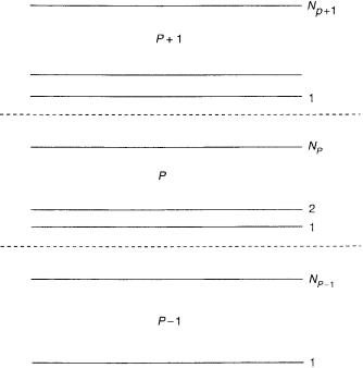
2.The range of the Pth sub-space is defined in such a way that the lowest (or the first) state and the highest (the NPth) state that belong to this subspace form Demkov-type interactions with the highest state belonging to the lower (P 1)th sub-space and with the lowest state belonging to the upper (P þ 1)th sub-space, respectively (see Fig. 2). In other words, the two non-adiabatic coupling terms fulfill the conditions:

At this point, we make two comments: (a) Conditions (1) and (2) lead to a well-defined sub-Hilbert space that for any further treatments (in spectroscopy or scattering processes) has to be treated as a whole (and not on a ‘‘state by state’’ level). (b) Since all states in a given sub-Hilbert space are adiabatic states, strong interactions of the Landau–Zener type can occur between two consecutive states only. However, Demkov-type interactions may exist between any two states.

B.The Construction of Sub-Sub-Hilbert Spaces

As we have seen, the sub-Hilbert spaces are defined for the whole configuration space and this requirement could lead, in certain cases, to situations where it will be necessary to include the complete Hilbert space. However, it frequently happens that the dynamics we intend to study takes place in a given, isolated, region that contains only part of the conical intersection points and the question is whether the effects of the other conical intersections can be ignored?

The answer to this question can be given following a careful study of these effects employing the line integral approach presented in terms of Eq. (27). For this purpose, we analyze what happens along a certain line that surrounds

Figure 2. A schematic picture describing the three consecutive sub-Hilbert spaces, namely, the (P 1)th, the Pth, and the (P þ 1)th. The dotted lines are separation lines.

one or several conical intersections. To continue, we employ the same procedure as discussed in Section IV.B: We break up the adiabatic-to-diabatic transformation matrix A and the s matrix as written in Eq. (43). In this way, we can show that if, along the particular line , the noninteresting parts of the s matrix are of order e the error expected for the interesting part in the A matrix is of order Oðe2Þ [81]. If this happens for any contour in this region, then we can ignore the effects of conical intersection that are outside this region and carry out the dynamic calculations employing the reduced set of states.

VII. THE TOPOLOGICAL SPIN

Before we continue and in order to avoid confusion, two matters have to be clarified: (1) We distinguished between two types of Landau–Zener situations, which form (in two dimensions) the Jahn–Teller conical intersection and the Renner–Teller parabolical intersection. The main difference between the two is

that the parabolical intersections do not produce topological effects and therefore, as far as this subject is concerned, they can be ignored. Making this distinction leads to the conclusion that the more relevant magnitude to characterize topological effects, for a given sub-space, is not its dimension M but NJ , the number of conical intersections. (2) In general, one may encounter more than one conical intersection between a pair of states [12,22,26,66,74]. However, to simplify the study, we assume one conical intersection for a pair of states so that ðNJ þ 1Þ stands for the number of states that form the conical intersections.

So far, we introduced three different integers M, NJ , and K. As mentioned earlier, M is a characteristic number of the sub-space (see Section VI.B) but is not relevant for topological effects; instead NJ , as just mentioned, is a characteristic number of the sub-space and relevant for topological effects, and K, the number of ( 1) terms in the diagonal of the topological matrix D (or the number of eigenstates that flip sign while the electronic manifold traces a closed contour) is relevant for topological effects but may vary from one contour to another, and therefore is not a characteristic feature for a given sub-space.

Our next task is to derive all possible K values for a given NJ . First, we refer to a few special cases: It was shown before that in case of NJ ¼ 1 the D matrix contains two ( 1) terms in its diagonal in case the contour surrounds the conical intersection and no ( 1) terms when the contour does not surround the conical intersection. Thus the allowed values of K are either 2 or 0. The value K ¼ 1 is not allowed. A similar inspection of the case NJ ¼ 2 reveals that K, as before, is equal either to 2 or to 0 (see Section V.B). Thus the values K ¼ 1 or 3 are not allowed. From here, we continue to the general case and prove the following statement:

In any molecular system, K can attain only even integers in the range [9]:

where p is an integer.

The proof is based on Eq. (87). Let us assume that a certain closed contour yields a set of aij angles that produce a number K. Next, we consider a slightly different closed contour, along which one of these aij parameters, say ast, changed its value from zero to p. From Eq. (87), it can be seen that only two D matrix elements contain cosðastÞ, namely, Dss and Dtt. Now, if these two matrix elements were positive following the first contour, then changing ast from 0 ! p would produce two additional ( 1) terms, thus increasing K to K þ 2; if these two matrix elements were negative, this change would cause K to decrease to K 2; and if one of these elements was positive and the other negative, then