

Baer M., Billing G.D. (eds.) - The role of degenerate states in chemistry (Adv.Chem.Phys. special issue, Wiley, 2002)
.pdfthe electronic non-adiabatic coupling term |
113 |
B.The Study of a Real Three-State Molecular System: Strongly Coupled
(2,3) and (3,4) Conical Intersections
We ended Section XV.A by claiming that the value að j q ¼ 0:4 A˚Þ is only 0.63p instead of p (thus damaging the two-state quantization requirement) because, as additional studies revealed, of the close locations of two (3,4) conical intersections. In this section, we show that due to these two conical intersections our sub-space has to be extended so that it contains three states, namely, the second, the third, and the fourth states. Once this extension is done, the quantization requirement is restored but for the three states (and not for two states) as will be described next.
In Section IV, we introduced the topological matrix D [see Eq. (38)] and showed that for a sub-Hilbert space this matrix is diagonal with (þ1) and ( 1) terms a feature that was defined as quantization of the non-adiabatic coupling matrix. If the present three-state system forms a sub-Hilbert space the resulting D matrix has to be a diagonal matrix as just mentioned. From Eq. (38) it is noticed that the D matrix is calculated along contours, , that surround conical intersections. Our task in this section is to calculate the D matrix and we do this, again, for circular contours.
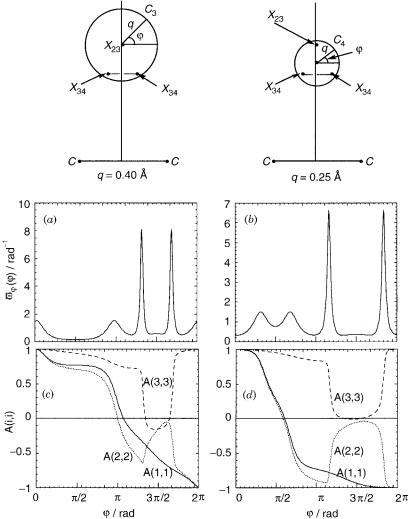
The numerical part is based on two circles, C3 and C4, related to two
˚
different centers (see Fig. 13). Circle C3, with a radius of 0.4 A, has its center at the position of the (2,3) conical intersection (like before). Circle C4, with a
˚ ˚
radius 0.25 A, has its center (also) on the C2v line, but at a distance of 0.2 A from the (2,3) conical intersection and closer to the two (3,4) conical intersections. The computational effort concentrates on calculating the exponential in Eq. (38) for the given set of ab initio 3 3 s matrices computed along the above mentioned two circles. Thus, following Eq. (28) we are interested in calculating the following expression:
j |
|
|
|
Aðj j qÞ ¼ } exp ð0 |
sjðj0 j qÞdj0 |
ð188Þ |
where value of q determines the circular contour. The matrix DðqÞ is, accordingly:
DðqÞ ¼ Aðj ¼ 2p j qÞ |
ð189Þ |
To calculate Aðj j qÞ the angular interval f0; jg is divided into n (small enough) segments with fj0ð¼ 0Þ; j1; . . . ; jnð¼ jÞg as division points, so that the A matrix can be presented as
Y |
ð |
|
|
! |
|
|
n |
1 exp |
|
jk |
sðj0Þdj0 |
|
|
Aðj ¼ jnÞ ¼ k |
|
jk 1 |
ð190Þ |
|||
¼ |
|
|
|
|
|
|
the electronic non-adiabatic coupling term |
115 |
where the variable q is deleted. By following the procedure described in [57], one presents AðjnÞ as
Yn
AðjnÞ ¼ GkyEðjkÞGk |
ð191Þ |
k¼1 |
|
where Gk is a unitary matrix that diagonalizes tðjÞ at the mid-point of the kth segment: j~k ¼ ðjk þ jk 1Þ=2 and EðjkÞ is a diagonal matrix with elements
ðm ¼ 1; 2; . . . ; MÞ:
|
ð |
jk |
1 |
|
|
EmðjkÞ ¼ exp |
|
jk þ |
tmðjÞdj! ¼ expð tmðj~kÞ jÞ |
ð192Þ |
|
~ |
|
|
~ |
j is the angular |
|
Here, tmðjÞ; m ¼ 1; 2; . . . ; M are the eigenvalues of tðjÞ and |
|||||
grid size. The order of the multiplication in Eq. (191) is such that the k ¼ 0 term is the first term from the right-hand side in the product. With these definitions the matrix D is defined as DðqÞ ¼ Aðj ¼ jN j qÞ, where jN ¼ 2p [see Eq. (189)].
Going back to our case and recalling that tðj j qÞ is a 3 3 antisymmetric matrix it can be shown that one of its eigenvalues is always zero and the others
are two imaginary conjugate functions, namely, ivðjÞ where vðjÞ ¼ p
t212 þ t223 þ t213. In Figure 13a and b we present vðjÞ functions as calculated
for the two circles C3 and C4 (see the relevant upper panels of Fig. 13). The two strong spikes are due to the two (3,4) conical intersections and they occur at points where the circles cross their axis line.
To perform the product in Eq. (191) we need the G matrices and, for this 3 3 matrix, these can be obtained analytically [7,80]. Thus
|
G |
|
1 |
|
|
it23v |
t13t12 |
it23v t13t12 |
|
t13lp2 |
|
193 |
||
|
|
|
|
|
|
it13v |
t23t12 |
it13v |
t23t12 |
t23l |
p |
|
|
|
|
|
|
vl |
|
B |
2 |
|
|
||||||
|
|
|
|
|
l2 |
l2 |
t12lp2 C |
ð Þ |
||||||
|
|
|
|
|
@ |
|
þ |
|
þ |
|
|
|
A |
|
|
|
¼ p2 |
0 |
|
|
|
1 |
|||||||
where l ¼ |
t232 þ t132 . |
|
|
|
|
|
|
|
||||||
In |
|
|
p |
we present the |
three diagonal |
elements |
of the |
|||||||
|
Figure 13c and d |
|||||||||||||
corresponding adiabatic-to-diabatic transformation matrices Aðj j qÞ as calculated for the two circles. Note that A11ðj j qÞ, in both cases, behaves smoothly while varying essentially undisturbed, from (þ1) to ( 1). The second diagonal term in each case, that is, A22ðj j qÞ, follows the relevant A11ðj j qÞ, until the contour enters the region of the (3,4) conical intersections. There the A22ðj j qÞ terms start to increase like they would do if only one (3,4) conical intersection were present. However, once they have reached the region of the second (3,4) conical intersection this conical intersection pushes the curve down again so that
116 michael baer
finally the A22ðj j qÞ terms become ( 1), instead of (þ1). The third term, A33ðj j qÞ in each case, proceeds undisturbed as long as it is out of the range of the two (3,4) conical intersections. Once it enters the region of the first conical intersection, the curve starts to decrease and eventually becomes ( 1) as it should if only one conical intersection was present. However, as the contour reaches the region of the second conical intersection, A33ðj j qÞ is pushed back and ends up with the value of (þ1), instead of ( 1). The value of each term Aiiðj ¼ 2p j qÞ; i ¼ 1; 2; 3 constitutes the diagonal of the D matrix for the particular contour:
|
˚ |
|
The results for C4ðq ¼ 0:25 AÞ are as follows: |
|
|
D11 ¼ 0:9998; |
D22 ¼ 0:9999; |
D33 ¼ 0:9997: |
|
˚ |
|
The results for C3ðq ¼ 0:4 AÞ are as follows: |
|
|
D11 ¼ 0:990; |
D22 ¼ 0:988; |
D33 ¼ 0:997: |
While studying these results we have to pay attention to two features: (1) In each case, these numbers must, in absolute value, be as close as possible to 1; and (2) two of these numbers have to be negative. Then, we also have to be able to justify the fact that it is the first two diagonal elements that have to be negative and it is the third one that must be positive. Note that these Dii terms are reasonably close to fulfilling the expected features just mentioned:
For the three relevant (absolute) numbers, the two different calculations yielded Djj values (three for each case) all in the range 0:99 jDjjj 0:9999— thus the quantization is fulfilled to a very high degree.
The values due to the two separate calculations are of the same quality we usually get from (pure) two-state calculations, that is, very close to 1.0 but two comments have to be made in this respect: (1) The quality of the numbers are different in the two calculations: The reason might be connected with the fact that in the second case the circle surrounds an area about three times larger than in the first case. This fact seems to indicate that the deviations are due ‘‘noise’’ caused by CIs belonging to neighbor states [e.g., the (1,2) and the (4,5) CIs].
(2) We would like to remind the reader that the diagonal element in case of the two-state system was only ( )0.39 [73] [instead of ( )1.0] so that incorporating the third state led, indeed, to a significant improvement.
The requirement of having two negative values and one positive is also fulfilled. Since this subject has been treated several times before (see Sections VIII and IX) it will be discussed within the next subject, related to the locations of the negative terms, that requires some analysis.
The positions of the ( 1) terms in the diagonal indicate which of the electronic eigenfunction flips sign upon tracing the closed contour under
the electronic non-adiabatic coupling term |
117 |
consideration [see Section (IV.A)]. The results of this study show that in both cases the eigenfunctions of the two lower states (i.e., 22A0 and 32A0) flip sign, whereas the sign of the third function (i.e., 42A0) remains the same. In situations where we have a single conical intersection between each consecutive pair of states it is the first and the third eigenfunctions that flip sign (see Section VIII). Here, we encounter the situation of one conical intersection between the lower pair of states but two (not one) conical intersections between the upper pair of states.
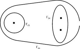
To analyze this case, we employ, as before, ‘‘contour algebra’’ (see Section IX): From Figure 14, it is noticed that 23 is a contour that surrounds the (2,3) conical intersection, 34 is the contour that surrounds the two (3,4) conical intersections, and 24 is a contour that surrounds all three conical intersections. According to ‘‘contour algebra’’ the event that ‘‘takes place’’ along 24 is the sum of the events along each individual contour. Thus,
24 ¼ 23 þ 34 |
ð194Þ |
Next, we are aware of the fact that if the system traces 23 it will be the two lower eigenfunctions that flip signs. If the system traces 34, then no function flips its sign because two such conical intersections cancel each other [12,22,26,74,125]. Now, if the system traces 24 then, from Eq. (194) it follows that again, only the two lowest functions flip their sign, so that the effect due to the single lower CI will be preserved. In other words, the two-state topological effects are not disturbed along those contours that surround all three CIs. The results will be different once we choose a contour that surrounds, in addition to the lower CI, only one of the two upper CIs [see Ref. (117b)].
Figure 14. The three contours for the three situations discussed in the text: 23 surrounds the (2,3) CI, 34 surrounds the two (3,4) CIs, and 24 surrounds all three CIs.
118 |
michael baer |
XVI. SUMMARY AND CONCLUSIONS
This field currently differs from others fields in molecular physics mainly in two ways: (1) It is a highly theoretical field and as such it requires chemical–physical intuition and mathematical skill. (2) This field is still open to new developments that could significantly affect chemistry when treated on the molecular level. In this chapter, we tried to summarize the various findings related to this field and to give the reader its state of the art. Some of the subjects presented here were already discussed in previous reviews [8,13]. Still, due to last year’s intensive efforts, we managed to include several new issues—some of them may open new venues for more research in this field. Since, as mentioned, part of the subjects presented here were already summarized in a previous review [13], in this section we will mainly concentrate on the implications of new subjects thus avoiding unnecessary repetition. We distinguish between two kinds of topics: (1) Practical ones that are associated with the possibility of treating dynamical processes related to excited states, namely, the diabatization process. (2) Less practical ones, which are interesting from a theoretical point of view but with potential prospects.
We start summarizing our findings regarding diabatization. There is no doubt that diabatization is essential for any dynamical study that involves electronically excited states. Diabatization is applied (on and off) for almost three decades mainly for studying charge-transfer processes between ion and molecules [54,94–97,125,127–131] and sporadically for other purposes [100– 104]. However, only recently the conditions for a correct diabatization, subject to minimal numerical efforts, were formulated [108]. This subject is discussed in Section XI. The diabatization as presented here is shown to be closely connected with the fact that the non-adiabatic coupling matrix has to be quantized to guarantee single-valued diabatic potentials. One of the more fundamental answers regarding the quantization of the nonadiabatic coupling matrix were given in a series of ab initio calculations for different molecules [64–74]. The quantization for two-state systems for real systems was discussed in our previous reviews [8,13] but here, in Section XV.B, we extended the discussion to a three-state case found to exist for the second, third, and fourth states of the C2H molecule [117]. This study is particularly important because it produces, for first time, the proof that the quantization is a general feature that goes beyond the two-state systems.
The two other subjects, as we already mentioned, are more theoretical but eventually may lead to interesting practical findings.
In Section XIII, we made a connection between the curl condition that was found to exist for Born–Oppenheimer–Huang systems and the Yang–Mills field. Through this connection we found that the non-adiabatic coupling terms can be considered as vector potentials that have their source in pseudomagnetic
the electronic non-adiabatic coupling term |
119 |
fields defined along seams. We speculated that these fields could be, semiclassically, associated with the zero-point vibrational motion [113].
Another subject with important potential application is discussed in Section XIV. There we suggested employing the curl equations (which any Bohr– Oppenheimer–Huang system has to obey for the for the relevant sub-Hilbert space), instead of ab initio calculations, to derive the non-adiabatic coupling terms [113,114]. Whereas these equations yield an analytic solution for any two-state system (the abelian case) they become much more elaborate due to the nonlinear terms that are unavoidable for any realistic system that contains more than two states (the non-abelian case). The solution of these equations is subject to boundary conditions that can be supplied either by ab initio calculations or perturbation theory.
This chapter centers on the mathematical aspects of the non-adiabatic coupling terms as single entities or when grouped in matrices, but were it not for the available ab initio calculation, it would have been almost impossible to proceed thus far in this study. Here, the ab initio results play the same crucial role that experimental results would play in general, and therefore the author feels that it is now appropriate for him to express his appreciation to the groups and individuals who developed the numerical means that led to the necessary numerical outcomes.
APPENDIX A: THE JAHN–TELLER MODEL AND THE
LONGUET–HIGGINS PHASE
We consider a case where in the vicinity of a point of degeneracy between two electronic states the diabatic potentials behave linearly as a function of the coordinates in the following way [16–21]
W ¼ k |
y |
|
x |
ðA:1Þ |
x |
|
y |
||
|
|
|
|
where (x; y) are some generalized nuclear coordinates and k is a force constant. The aim is to derive the eigenvalues and the eigenvectors of this potential matrix. The eigenvalues are the adiabatic potential energy states and the eigenvectors form the columns of the adiabatic-to-diabatic transformation matrix. In order to perform this derivation, we shall employ polar coordinates (q,j), namely,
y ¼ q cosj |
and |
x ¼ q sinj |
ðA:2Þ |
By substituting for x and y, we get j-independent eigenvalues of the form |
|||
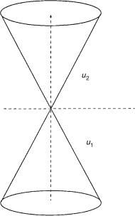
u1 ¼ kq and u2 ¼ kq |
where |
q ¼ f0; 1g and |
j ¼ f0; 2pg |
120 |
michael baer |
Figure 15. The two interacting cones within the Jahn–Teller model.
As noticed from Figure 15, the two surfaces u1 and u2 are conelike potential
energy surfaces with a common apex. The corresponding eigenvectors are |
|
|
||||||||||
|
¼ |
j |
|
j |
|
A:3 |
|
|||||
f1 |
cos |
j |
; |
sin |
j |
|
|
|
|
|||
|
|
2 |
|
2 |
|
ð |
|
Þ |
||||
f2 |
¼ sin |
|
; |
cos |
|
|
|
|||||
2 |
2 |
|
||||||||||
The components of the two vectors (n1, n2), when multiplied by the electronic (diabatic) basis set (jf1i; jf2i), form the corresponding electronic adiabatic basis set ðjZ1i; jZ2iÞ:
|
|
j |
j |
|
|||
jZ1i ¼ cos |
|
|
|
jf1i þ sin |
|
jf2i |
|
|
2 |
2 |
ðA:4Þ |
||||
|
j |
j |
|||||
jZ2i ¼ sin |
|
jf1i cos |
|
jf2i |
|
||
2 |
2 |
|
|||||
The adiabatic functions are characterized by two interesting features: (1) they depend only on the angular coordinate (but not on the radial coordinate) and
(2) they are not single valued in configuration space because when j is replaced by (j þ 2p)—a rotation that brings the adiabatic wave functions back to their
the electronic non-adiabatic coupling term |
121 |
initial position—both of them change sign. This last feature, which was revealed by Longuet-Higgins [14–17], may be, in certain cases, very crucial because multivalued electronic eigenfunctions cause the corresponding nuclear wave functions to be multivalued as well, a feature that has to be incorporated explicitly (through specific boundary conditions) while solving the nuclear Schro¨dinger equation. In this respect, it is important to mention that ab initio electronic wave functions indeed, possess the multivaluedness feature as described by Longuet–Higgins [30].
One way to eliminate the multivaluedness of the electronic eigenfunctions is by multiplying it by a phase factor [15], namely,
zjðjÞ ¼ expðiWÞZjðjÞ j ¼ 1; 2 |
ðA:5Þ |
where a possible choice for W is
W ¼ j=2 |
ðA:6Þ |
Note that zjðjÞ; j ¼ 1; 2 are indeed single-valued eigenfunctions; however, instead of being real, they become complex.
The fact that the electronic eigenfunctions are modified as presented in Eq. (A.5) has a direct effect on the non-adiabatic coupling terms as introduced in Eqs. (8a) and (8b). In particular, we consider the term tð111Þ (which for the case of real eigenfunctions is identically zero) for the case presented in Eq. (A.5):
s11ð1Þ ¼ hz1jrz1i ¼ irW þ hZ1jrZ1i |
|
but since |
|
hZ1jrZ1i ¼ 0 |
|
it follows that s11ð1Þ becomes |
|
s11ð1Þ ¼ irW |
ðA:7Þ |
In the same way, we obtain |
|
s11ð2Þ ¼ ir2W ðrWÞ2 |
ðA:8Þ |
The fact that now sð111Þ is not zero will affect the ordinary Born–Oppenheimer approximation. To show that, we consider Eq. (15) for M ¼ 1, once for a real

122 |
michael baer |
eigenfunction and once for a complex eigenfunction. In the first case, we get from Eq. (15) the ordinary Born–Oppenheimer equation:
|
1 |
ðA:9Þ |
2m r2c þ ðu EÞc ¼ 0 |
because for real electronic eigenfunctions sð111Þ 0 but in the second case for which sð111Þ ¼6 0 the Born–Oppenheimer approximation becomes
|
1 |
ðr þ irWÞ2c þ ðu EÞc ¼ 0 |
ðA:10Þ |
2m |
which can be considered as an ‘extended’ Born–Oppenheimer approximation for a case of a single isolated state expressed in terms of a complex electronic eigenfunction [132]. This equation was interpreted for some time as the adequate Schro¨dinger equation to describe the effect of the conical intersection that originate from the two interacting states. As it stands it contains an effect due to an ad hoc phase attached to a ground-state electronic eigenfunction [63].
The extended Born–Oppenheimer approximation based on the nonadiabatic coupling terms was discussed on several occasions [23,25,26,55,56,133,134] and is also presented here by Adhikari and Billing (see Chapter 3).
APPENDIX B: THE SUFFICIENT CONDITIONS FOR HAVING
AN ANALYTIC ADIABATIC-TO-DIABATIC
TRANSFORMATION MATRIX
The adiabatic-to-diabatic transformation matrix, Ap, fulfills the following firstorder differential vector equation [see Eq. (19)]:
$AM þ tMAM ¼ 0 |
ðB:1Þ |
In order for AM to be a regular matrix at every point in the assumed region of configuration space it has to have an inverse and its elements have to be analytic functions in this region. In what follows, we prove that if the elements of the components of tM are analytic functions in this region and have derivatives to any order and if the P subspace is decoupled from the corresponding Q subspace then, indeed, AM will have the above two features.
I.ORTHOGONALITY
We start by proving that AM is a unitary matrix and as such it will have an inverse (the proof is given here again for the sake of completeness). Let us consider the