Baer M., Billing G.D. (eds.) - The role of degenerate states in chemistry (Adv.Chem.Phys. special issue, Wiley, 2002)

approximation whereas, for degenerate or nearly degenerate states, it results into the vibronic Hamiltonian that allows the nonadiabatic mixing of electronic states having the same or close energies. First, let us examine the case of a nondegenerate electronic state cnðr; s; RÞ. To first order of degenerate perturbation theory, this is equivalent to considering just the diagonal elements of the Hamiltonian matrix HðR0; iÞ or to neglecting all terms in Eq. (3) but the nth one

Thus, the neglect of the off-diagonal matrix elements allows the change from mixed states of the nuclear subsystem to pure ones. The motion of the nuclei leads only to the deformation of the electronic distribution and not to transitions between different electronic states. In other words, a stationary distribution of electrons is obtained for each instantaneous position of the nuclei, that is, the electrons follow the motion of the nuclei adiabatically. The distribution of the nuclei is described by the wave function wnðR0; iÞ in the potential Vnn þ Cnn, known as the proper adiabatic approximation [41]. The off-diagonal operators Cmn in the matrix C, which lead to transitions between the states cn and cm, are called operators of nonadiabaticity and the potential Vn ¼ VnnðRÞ due to the mean field of all the electrons of the system is called the adiabatic potential.

To obtain the Hamiltonian at zeroth-order of approximation, it is necessary not only to exclude the kinetic energy of the nuclei, but also to assume that the nuclear internal coordinates are frozen at R ¼ R0, where R0 is a certain reference nuclear configuration, for example, the absolute minimum or the conical intersection. Thus, as an initial basis, the states cnðr; sÞ ¼ cnðr; s; R0Þ

n

Substitution of Eq. (12) into the Schro¨dinger equation leads to a system of coupled differential equations similar to Eq. (5), but with the following differences: the potential matrix with elements

is nondiagonal in the new basis, whereas the matrix of the kinetic energy operator for the nuclei vanishes as the basis functions do not depend on R. For the nondegenerate state case, one has to take into account only the diagonal elements of the Hamiltonian,

where Vnn plays the role of the potential energy of the nuclei. This is equivalent to looking for solutions of the form in Eq. (11). If a complete basis set is assumed, the eigenvalues of the potential matrix then coincide with the adiabatic potentials Vn from Eq. (4).

This approach is called the Born–Oppenheimer (BO) approximation [38]. It is linked to the proper adiabatic approximation by the unitary transformation of the electronic basis and from this point of view they are equivalent. Of course, such an equivalence is valid only for exact solutions. In fact, the convergence of approximate solutions is different for those two cases. In particular, the BO approximation necessarily involves the expansion of the potential energy in a power series with respect to nuclear displacements from the point R0, and hence leads to a different convergence when compared with the adiabatic approximation. In some cases though, the weak convergence or even nonvalidity of the BO approximation is caused not by the large contribution of the operator of nonadiabaticity but by the signficant anharmonicity of the potential energy surface, especially in the case of nonrigid molecules where the adiabatic approximation may possibly work. On the other hand, the BO approximation is convenient since it allows the use of symmetry considerations due to the fact that the electronic states fcnðrÞg form the basis of irreducible representations (IRREPs) of the symmetry group appropriate to the nuclear configuration R0.

However, for some polyatomic systems, there are electronic states for which the adiabatic and the BO approximations are inapplicable. In such cases, the electronic term energies are very close or coincide at some number (finite or infinite) of points of the configurational space of the nuclei. Such a degeneracy of the terms in the electronic subsystem is usually due to the high symmetry of the nuclear configuration at the point R0. This is the case, for example, when the potential energy surface shows a conical intersection. As a result of such degeneracies, the BO approximation described in the previous paragraph breaks down. In fact, as first pointed out by Longuet-Higgins and Herzberg [42– 44], due to such a conical intersection, a real electronic wave function changes sign when traversing a nuclear path that encircles the degeneracy point. On the other hand, the total electronuclear wave function must be continuous and single-valued, which implies that the nuclear wave function must change sign to compensate that of the electronic wave function. This may be achieved by introducing a geometry-dependent phase factor in the Born–Huang [39] type

where cnðr; s; RÞ are the real-valued solutions of Eq. (4), and the AnðRÞ are

n

where the complex nuclear wave functions w~nðR0; iÞ are now chosen to makeðR0; i; r; sÞ be single valued. Clearly, the R dependence of AnðRÞ must reflect the presence of any conical intersection in accordance with the Berry phase condition, and hence can generally be constructed only after the conical intersections have been located. Although a general approach for determining AnðRÞ has been suggested by Kendrick and Mead [45], it remains a nontrivial task. As shown in Appendix A, a simpler approach is possible if one assumes a two-dimensional (2D) Hilbert space model, that is, only two electronic states.

Mead and Truhlar [19,46,47] showed that the ansatz of Eq. (15) leads to the appearance of a vector potential in the nuclear Schro¨dinger equation. For a X3-type molecule, the same result can be achieved by multiplying the real nuclear wave function by a complex phase factor such that it changes sign on encircling the conical intersection, and hence makes the resulting complex nuclear wave function single valued [48–50]. Billing and Markovic [51] adopted hyperspherical coordinates within this complex phase factor approach to include such a GP effect in X3 molecules that have a single D3h conical intersection, since in this coordinate system the GP effect concerns in principle only the f hyperangle. A similar approach has been utilized by the present authors [2] to study the transition state resonances and bound vibrational states of H3 using a time-dependent wavepacket method. Because all the above methods still use only one electronically adiabatic potential energy surface, they can be said to be based on a generalized BO approximation [52]. Within this spirit, we have also reported [4], following the approach of Baer and Englmann [53] and Xu et al. [5], a generalized BO equation [4] to study the nuclear dynamics in the vicinity of the conical intersection (see Appendix A). Such studies on both the electronically ground doublet state [11] and firstexcited doublet state [12] of trimeric hydrogenic systems have shown that the GP effect plays a significant role, and should be taken into account if accurate dynamics results are aimed.

III.GROUP THEORETICAL CONSIDERATIONS

As is well known, when the electronic spin–orbit interaction is small, the total electronic wave function ceðr; s; RÞ can be written3 as the product of a spatial wave function c0eðr; RÞ and a spin function cesðsÞ. For this, we can use either

3 Although for a Slater-type determinant wave function this is true only for two-particle systems, the following discussion is independent of such a restriction.

the SF or the BF coordinate systems. As shown below, it is more appropriate to use BF spin functions, since they will be affected by molecular symmetry operations, and hence must belong to one of the irreducible representations of the symmetry point group of the molecule. For example, for integer spin values, the transformation expðimSjÞ for rotation by j ¼ 2p, where mS ¼ S; S 1; . . . ; S, leads to a retrieval of the spin function to itself [28]. However, when the spin is a half-integer, such a transformation (i.e., a rotation by 2p) will lead to a sign change of the spin function. Indeed, if j0 ¼ j þ 2p and mS ¼ l=2, where l is an integer, one has expðimSj0Þ ¼ expðimSjÞ. The spin function will then be double valued: A rotation by 2p will not bring the system to its starting point, which can only be achieved through a 4p rotation. A rotation by 2p is therefore a new symmetry element, called R (to denote the corresponding

Such extended point groups are commonly referred to as double groups [28], and we give some examples in Table I; the dashed lines on this table indicate the separation between the traditional point group and its extension. Note that, for

belong to the same class as the original elements and cause only a doubling of the class. For axes more than twofold and the center of symmetry, they cause a

Herzberg’s [28] book.

Note also that on reducing the symmetry of a system, the spin functions for integer spin are resolved by reducing degeneracies [28]. In simple words, this means that by reducing the symmetry, the degenerate spin states in the highsymmetry group split into different states in the lower symmetry group. However, the spin functions for half-integer spin are at most resolved into functions that are still doubly degenerate. Indeed, we may see from Table II that, for integer total electronic spin S or integer total nuclear spin I, on going from D3h to C2v the E00 representation transforms to B1 þ B2. Conversely, for the S or I half-integer, the same resolution maintains the E-type degenerate representation. This remaining degeneracy is usually called Kramers’ degeneracy to honor the author who first discovered it [28,30]. According to Kramers’ theorem, provided that no external magnetic field is present, the degeneracy of a system consisting of an odd number of identical particles with half-integer spin (fermions) is even. This is due to the fact that, as long as no magnetic field is present, there is in all atomic and molecular systems an additional symmetry

As usual, the indices 1=2, 3=2, and 5=2 that appear in the doubly degenerate E representation indicate the values of the projection of the angular momentum vector, mJ ¼ 1=2; 3=2; 5=2; see also the text.

^

element that corresponds to the antilinear time reversal operator T (see Appendix B): The evolution of a system (classical or quantum) is invariant when the time t is replaced by t. In fact, an extension of Kramers’ theorem will be demonstrated to be valid also for systems with a half-integer total angular momentum quantum number F.

Consider then the total angular momentum F defined by the vectorial sum of all the angular momenta of the system

where S; I; L, and N are the total electronic spin, nuclear spin, electronic orbital angular momentum, and nuclear orbital angular momentum. For this general case, we can prove that Kramers’ theorem still applies since spin and orbital angular momenta must obey the same time-reversal properties (see Appendix C), namely,

^

where A represents as usual the operator corresponding to the angular momentum (vector) A, while the quantum number A defines the eigenvalue

Equations (18)–(22) imply that all types of angular momenta have the same timereversal properties. In fact, it is well known [54,55] that quantities such as energy, coordinates, electric field strength, and so on are invariant under time reversal: The corresponding operators must be time invariant. In turn, the velocity, linear momentum, angular momentum, magnetic field strength, and so on, change sign under time reversal: The corresponding operators must reflect the same property.

Moreover, as also shown in Appendix C for the electronic spin, one has

^

where hereafter the operator TA stands for a time-reversal operation on the A variable. Similarly, for the nuclear spin, one has

and hence mutually commute. Note especially that L and N always assume integer values.

At this stage, we are ready to prove that Kramers’ theorem holds also for the total angular momentum F. We will do it by reductio ad absurdum. Then, let

Suppose now that the total wave function (state) is nondegenerate, and F is halfinteger. From Eq. (29), it then follows

where c is a constant, and hence

674 a. j. c. varandas and z. r. xu

Finally, we can demonstrate that the degeneracy is even when the total angular momentum quantum number F is half-integer, again via a reductio ad absurdum method. Suppose that the degeneracy of the eigenstates is k, then we have k degenerate states j E;ii ði ¼ 1; . . . ; kÞ, which have in common the same eigenvalue E. One can then form orthogonal pairs of such states such as j Ei

^j Ei. If k is odd, there will be a single state (e.g., jfi), which has no pair.

T

and

^jfi

However, as mentioned above, T will be orthogonal to all the k states, and

^jfi

T is nonzero. This implies that the number of total states of the same eigenvalue E is ðk þ 1Þ, which contradicts our initial hypothesis. Thus, we conclude that k must be even, and hence proved the generalized Kramers’ theorem for total angular momentum. The implication is that we can use double groups as a powerful means to study the molecular systems including the rotational spectra of molecules. In analyses of the symmetry of the rotational wave function for molecules, the three-dimensional (3D) rotation group SOð3Þ will be used.

IV. PERMUTATIONAL SYMMETRY OF

TOTAL WAVE FUNCTION

^ ^

The total Hamiltonian operator H must commute with any permutations PX among identical particles (X) due to their indistinguishability. For example, for a system including three types of distinct identical particles (including

distinct sets of identical particles, there must be N such commutative laws similar to those in Eq. (46), which are relative to the various kinds of permutations; thus, there will be N permutational restrictions on the total wave function ðR0; i; r; sÞ. Note from Figures 1d and 2 that under the permutation of two identical nuclei, the hyperspherical coordinates for a three-particle system transform as ðr; y; f; a; b; gÞ ! ðr; y; f; a; b; g þ pÞ.

We will now explain the meaning of the word ‘‘identical’’ used above. Physically, it is meant for particles that possess the same intrinsic attributes, namely, static mass, charge, and spin. If such particles possess the same intrinsic attributes (as many as we know so far), then we refer to them as physically identical. There is also another kind of identity, which is commonly referred to as chemical identity [56]. As discussed in the next paragraph, this is an important concept that must be stressed when discussing the permutational properties of nuclei in molecules.

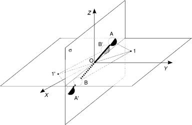
Figure 2. The space-fixed (XYZ ) and body-fixed (xyz) frames in a diatomic molecule AB. The nuclei are at A and B, and 1 represents the location of a typical electron. The results of inversions of their SF coordinates are A ! A0, B ! B0, and 1 ! 10, respectively. After one executes only the reinversion of the electronic SF coordinates, one obtains 10 ! 1. The net effect is then the exchange of the SF nuclear coordinates alone.

Then, let us first examine 7Li3 in a D3h structure. In this molecule, the three nuclei not only have the same intrinsic attributes but also have the same molecular environments due to the fact that they are in chemically equivalent positions. Thus, the three nuclei can be exchanged by rotations of the molecule and the permutational symmetry requirement must be satisfied. Now, consider a molecule like methanol (CH3OH) with four physically identical hydrogens. For any conformation, the methyl hydrogens will be distinguishable from one another through their positions relative to that of the hydroxyl hydrogen. However, the barrier for internal rotation of CH3 around the CO axis is low, and tunneling from one equivalent conformation to another may occur. Thus, the permutational symmetry requirement must be applied to the methyl hydrogens. A third example is the linear conformation of NNO, with two physically identical nitrogen nuclei. In principle, the permutational symmetry requirement should also be applied to the two 14N nuclei since they are physically identical. However, the two nuclei are placed at different molecular environments, that is, one lies adjacent to the oxygen nucleus while the other does not. Since their permutation involves an extremely high energy process, we may regard such nitrogen nuclei as distinguishable. They can then be said to be chemically nonequivalent [56], and hence not subject to the permutational symmetry