Baer M., Billing G.D. (eds.) - The role of degenerate states in chemistry (Adv.Chem.Phys. special issue, Wiley, 2002)

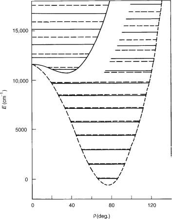
608 miljenko peric´ and sigrid d. peyerimhoff

corresponding to all possible K quantum numbers, with the spacing between successive sublevels being much smaller than that between neighboring vibrational levels, and increasing roughly quadratically with an increase of K. This structure corresponds to the Hamiltonian consisting of the sum of operators for a one-dimensional (1D) harmonic oscillator and a 1D free rotator with the moment of inertia I ¼ 1=mr2e , where re represents the equilibrium value of the bending coordinate r for the state in question. The gradual transformation of the Hamiltonian we use is easy to explain: First, if we change the volume element from rdr (as asummed above) into dr, the term in the kinetic energy operator involving the first derivative of r [for the following qualitative analysis it suffices to consider its simple form given by Eq. (5)] disappears; in the region around the equilibrium geometry of a bent state the molecule vibrates with small amplitudes so that we can replace r in the expression 1=r2 by re. Thus the

linearity is small and regular (Hund’s case b).

With increasing quantum number u, that is, by approaching the barrier to linearity, the spacing between vibrational levels generally diminishes, reaching minimum in the vicinity of the barrier, as first observed by Dixon [35]. At the same time, the K pattern becomes irregular, reflecting the gradual change of the rotational structure of the bent molecule into the linear molecule vibrational structure. The most spectacular manifestation of this is that at the energy close to that of the joint point of two adiabatic potentials, the K ¼ 1 level of the lower electronic state falls below its K ¼ 0 counterpart corresponding to the same quantum number u (see also [8] and [24]).

A consequence of the reordering of vibronic levels described above is the ambiguity concerning the definition of the bending vibrational frequency and the corresponding quantum number u (one should not wonder about that; such problems are always possible when one uses ‘‘bad’’ quantum numbers; more seriously, the quantum numbers not exactly determining the eigenvalues of the complete Hamiltonian of the system considered). In a bent molecule, the vibrational frequency is (nearly) equal to the separation of two neighboring levels with the same rotational quantum number. In a linear molecule this energy difference is divided by 2. What about the energy region around the barrier? Formally, the problem could be solved by accepting either the former or the latter definition and by employing it consequently. We can label each series of K levels beginning from the lowest one with the running number u. This is what is called ‘‘bent notation’’ (ub2 in Fig. 6). However, if we do that, we have the situation that above the barrier to linearity the energy difference between the vibronic levels with the same quantum number u (and different K) is comparable to the bending frequency. But the main role of a quantum number

associated with the Hamiltonian is just to give at least rough information about the energy of the level labeled by it. That is the reason that besides this ‘‘bent notation’’ the ‘‘linear notation’’ is also employed, the latter one assuming a 2D harmonic oscillator as the zeroth-order problem. In Figure 6, we label in this way (ul2) the levels of the upper electronic state. Note that the problem with two notations, none of them being universally satisfactory, is a consequence of large-amplitude bending vibrations the in course of which a molecule with bent equilibrium geometry passes though the linear nuclear configuration, and thus appears also in electronic states ( ) not exhibiting the R–T effect. The relationship between the vibrational quantum numbers is simple, ulin2 ¼ 2 ub2 þ jlj (in order to avoid confusion with the quantum number l we use here superscript ‘‘lin’’ for ‘‘linear’’), but unfortunately they are many papers in which it has not been explicitly quoted which notation has been meant.

In the upper electronic state, the BH2 molecule has linear equilibrium geometry. This has as a consequence a peculiar vibronic structure: The lowest lying level belonging to this state is a K ¼ 0 species with the energy of 2o (linear notation). That is so, because it correlates with the lowest lying l ¼ 1 (ulin ¼ 1) vibrational level. This fact has been overlooked in early ab initio studies on BH2 [36], which has contributed to the misstatement that the theory has failed to reproduce the experimental findings reliably [37] in this apparently simple case (with only seven electrons, BH2 is the smallest polyatomic molecule whose spectrum has been analyzed in detail thus far). On the other hand, the upper electronic state of NH2 shows a typical example of quasilinearity, with a single vibrational level lying below the joint point of adiabatic electronic states at linear geometry.

An important difference between the weak and strong R–T effect is that in the latter case there are no levels with clearly pronounced unique character. Instead, for each K ¼6 0 value there are several levels in the energy region around the joint point of the potential surfaces that share among themselves the unique character, in the sense, for example, that their spin–orbit splitting, while being much smaller than the value of the spin–orbit coupling constant, is appreciably larger than that for the levels that belong predominantly to a particular adiabatic electronic state. This is reflected in Figure 6 by missing of the u2 ¼ 0, K ¼ 1 vibronic level attributed to the upper electronic state.

As mentioned above, the R–T coupling in the systems with one or both adiabatic electronic states having bent equilibrium geometry is in general pronounced only in the neighborhood of the joint point of the potential surfaces. The exception represents the cases when a vibrational level belonging to the lower potential surface lies accidentally close to a counterpart of the upper electronic state. Note that ‘‘pragmatic’’ approaches that use pure ab initio calculated potential surfaces (as, e.g., those employed by the present authors) generally fail to describe such Fermi-type (local) interactions reliably, because

the restricted accuracy of the potential surfaces (errors of typically several hundred reciprocal centimeters) and neglect or approximate handling of some interactions (e.g., bend-stretch) consequently have inherent underor overestimating of the energy gap between such levels [16,17].

C.Choice of Hamiltonian

We find it convenient to reverse the historical ordering and to start with (nearly) exact nonrelativistic vibration–rotation Hamiltonians for triatomic molecules. From the point of view of molecular spectroscopy, the optimal Hamiltonian is that which maximally decouples from each other vibrational and rotational motions (as well different vibrational modes from one another). It is obtained by employing a molecule-bound frame that takes over the rotations of the complete molecule as much as possible. Ideally, the only remaining motion observable in this system would be displacements of the nuclei with respect to one another, that is, molecular vibrations. It is well known, however, that such a program can be realized only approximately by introducing the Eckart conditions [38].

Xn

A¼1

where mA represents the mass of the nucleus A, rA is the instantaneous position, and r0A its equilibrium position in the moving frame. The parameter n is the number of nuclei. The fulfillment of condition (33) ensures decoupling of vibrations from rotations (only) at infinitesimal vibrations. The corresponding quantum mechanical vibration–rotation Hamiltonian in terms of the (vibrational) normal coordinates was derived by Wilson et al. [39,40], and simplified by Watson [41,42]; we shall refer to it as the EWW Hamiltonian. It has (for molecules with nonlinear equilibrium geometry) the form

H¼ 1 X mabðJa pa La SaÞðJa pa La SaÞ

2 a;b

where mab1 (a; b ¼ x; y; or z) represents the element of a matrix that is nearly equal to the instantaneous moment of inertia matrix; Ja; pa; La; Sa are the components of the total, vibrational, electronic, and spin angular momentum operator respectively; Pr is the momentum conjugate with the normal coordinates Qr; and V is the potential for vibrational motion expressed in terms of Qr. The natural handling of the corresponding Schro¨dinger equation is to expand mab and V in Taylor series in Qr about the equilibrium geometry and to apply the perturbation theory.

Use of the Hamiltonian where the vibrational and rotational motions, as well as different vibrational modes, are maximally decoupled from one another should be expected to enable the most consequent realization of the main idea followed in a theoretical, particularly ab initio treatment of the R–T effect, namely, to separate the variables in the Schro¨dinger equation as much as possible from one another before the actual computations are started. However, while the separation of the nuclear from electronic coordinates in the framework of the BO approximation is practically always carried out (at least as the starting point), the EWW scheme in not the only possible and often not even the most convenient for the treatment of the vibration–rotation problem. First, let us stress that the Eckart’s approach assumes the existence of a relatively deep minimum on the potential surface, being well separated from all other (local) minima. Second, the EWW Hamiltonian has the serious drawback that it has different forms for molecules with nonlinear and linear equilibrium geometry. Both of these facts cause difficulties in the description of quasilinear molecules. Furthermore, the nature of interaction between certain vibrational and rotational modes is sometimes such that they have to be treated simultaneously, as, for example, between the bending vibrations and the z-axis rotations in the R–T effect. It should also be mentioned that the form of the normal coordinates is not known in advance and that the transformation of the potential, normally computed as a function of some internal coordinates into the series in normal coordinates is complicated by the fact that the transformation from internal into normal coordinates is nonlinear for noninfinitesimal vibrations [43]. Application of the EWW formalism, being predestinated for a perturbative treatment, loses much of its attractiveness if one intends to solve the complete (or a part) of the vibration–rotation problem by a variational approach. Therefore, it is often advantageous to abandon the Eckart constraints and the use of normal coordinates in order to gain additional flexibility that can be utilized for designing more convenient forms for the particular parts of the Hamiltonian (e.g., to avoid some unpleasant singularities in the vibrational Hamiltonian [44]); furthermore, this enables derivation of explicit analytical expressions for the vibrational–rotational Hamiltonian, as will be shown below. Although some of the disadvantages mentioned above have disappeared in the last few years (so Estes and Secrest [45] derived a unified variant of the Watson’s Hamiltonian valid for both nonlinear and linear molecules—the present authors are not able to judge whether it is correct; Wei and Carrington [46] recently presented an exact Eckart-embedded kinetic energy operator in bond coordinates for triatomic molecules; for a review of other various possibilities see, e.g., [47]), for the reasons mentioned above the complete EWW Hamiltonian seems to never have been used in handling the R–T effect.

An alternative form of exact nonrelativistic vibration–rotation Hamiltonian for triatomic molecules (ABC) is that used by Handy, Carter (HC), and

co-workers [48–51]. It is given in terms of the geometrically defined vibrational coordinates, we denote by r1, r2, and W. The parameter r1 is the instantaneous value of the distance between the nuclei A and B, r2 the distance between C and B, and W is the instantaneous ABC bond angle (W ¼ p r; this symbol should be not confused with the electronic angular coordinate y). The moleculefixed axes are defined such that the molecule lies in the zx plane with the x axis (being parallel to the axis) bisecting the ABC angle and the A nucleus lying in the positive zx quadrant. Thus the z axis coincides with the molecular axis at linear nuclear arrangements. The apparently arbitrary choice of the coordinate axes might look strange; it is not motivated by physical reasons, that is, it does not worry about the strength of the coupling between different motion modes. This becomes understandable in terms of a statement by HC: ‘‘. . . we are not interested in least squares fit procedures for the identification of spectra, and it is possible to label our states from the energies we obtain . . .’’ [50]. The origin of this Hamiltonian is not quite clear: In the first paper in which they used it [48], HC claimed that they had taken it over from Carney et al. [52] (and transformed to the volume element sin W dr1 dr2 dW, in our notation) The latter authors also mention Lai and Hagstrom, but the trace is lost somewhere in the library of Indiana University [53]. It is, however, of little importance who the actual author of this Hamiltonian is, because a derivation of such a vibration–rotation Hamiltonian for triatomic molecules employing the chain rule for transformation of the derivatives in Cartesian space-fixed coordinates into curvilinear internal coordinates, using the Podolsky approach [54] (see also [55]) for transforming the classical Hamiltonian in curvilinear coordinate into its quantummechanical counterpart, or a combination of both methods (see, e.g., [56]) is not a serious problem (even if it is carried out without the use of computer algebra). The real contribution of HC was to show how to solve the corresponding Schro¨dinger equation, particularly in the presence of vibronic coupling.

The (kinetic energy part of the) Hamiltonian we are speaking about can be written in the following form:

In Eq. (37) J, L, and S are the total, electronic, and spin angular momentum, respectively, all of them defined with respect to the molecule fixed-coordinate axes. In order to avoid problems with the anomalous commutation relations for the components of the total angular momentum, it is following Van Vleck [57] replaced in (37) by its counterpart with a negative sign. (Note that Handy and coworkers prefer to change the sign of J rather than signs of the internal momenta L and S, as suggested in the original paper by Van Vleck; for a discussion of this matter see [58] and [59].

The approaches for treating the vibration–rotation problem employing two types of Hamiltonians as described above lead to considerable computational requirements in larger molecules (already for a tetraatomic molecule the potential surface depends on six vibrational coordinates) and/or if some of the vibrational modes are characterized by large amplitudes. For this reason, another strategy is also applied. The vibrational modes are divided into two classes: to the first belong those that are accompanied by relatively small displacements of the nuclei and can easily be handled perturbationally (or even in the harmonic approximation); the second class is build by the vibrational modes for which a large-amplitude handling is necessary, so that they require a more sophisticated treatment. So, for example, in quasilinear molecules (particularly triatomics and tetraatomics, considered in the present study) the bending vibration(s) play(s) a special role. Quite frequently in electronic spectra one observes relatively long progressions in the bending mode, because the equilibrium angles could have very different values in various electronic states,

in contrast to the bond lengths, which generally vary less from state to state. This makes a large-amplitude treatment for the bending motion imperative, while the stretching motions can usually be assumed to occur with small amplitudes. Another peculiarity of the bending mode is its relation to the rotations: When a molecule during the bending vibrations approaches linear geometry, a gradual transformation of one of its rotational degrees of freedom into the degenerate bending vibration takes place. Both of these facts play crucial roles in the R–T effect. Such situations have motivated a number of authors to develop various methods in which the emphasis is placed on an accurate treatment of the effective bending problem, while the other nuclear modes are treated more or less conventionally. Among those, the greatest popularity enjoys the approach introduced for triatomic molecules by Hougen, Bunker and Johns (HBJ) [60] and developed further by Bunker and his coworkers, particularly Jensen [61–67].

In the formalism of Bunker et al., the so-called reference configuration plays the role that has the equilibrium configuration in the EWW scheme. It is characterized by fixed bond lengths and the variable valence angle, and is chosen such that the bending motion at each value of the bending coordinate r is minimally coupled with the stretching vibrations. This is achieved by introducing in addition to (33) (with the equilibrium configuration replaced by reference configuration) the Sayvetz [68] condition,

where ref stands for ‘‘reference.’’ In analogy with the EWW scheme, the molecular potential and the elements of the m-matrix are expanded around the reference configuration into Taylor series in the two stretching normal coordinates, with the coefficients depending on r,

[The appearance of the (normally small) linear term in V is a consequence of the use of reference, instead of equilibrium configuration]. Because the stretching vibrational displacements are of small amplitude, the series in Eqs. (40) should

converge quickly. The zeroth-order Hamiltonian is obtained by neglecting all but

P

the leading terms in these expansions, mrefab and V0ðrÞ þ 1=2 lrQ2r and has the

where Jr ¼ i q=qr and mrr is the inverse of the ‘‘reduced mass’’ for the large amplitude bending vibrations. The Hamiltonian (41) is an essentially 1D operator (in r). The coupling between r and the other degrees of freedom can be taken into account perturbationally [62,64], or indirectly as in the framework of the semirigid beneder model by Bunker and Landsberg [63], by allowing the bond lengths to vary smoothly with changes in r an by correcting correspondingly the potential V0ðrÞ.

D.Minimal Models

In his classical paper, Renner [7] first explained the physical background of the vibronic coupling in triatomic molecules. He concluded that the splitting of the bending potential curves at small distortions of linearity has to depend on r2 , being thus mostly pronounced in electronic state. Renner developed the system of two coupled Schro¨dinger equations and solved it for states in the harmonic approximation by means of the perturbation theory.

For a long time, Renner’s paper had been unique. There are two main reasons for this: There have been no reliable experimental results that could have confirmed Renner’s predictions and, on the other hand, this work has been carried out so thoroughly that there have been no reasons to try to improve it. The situation changed almost 25 years later, but it changed completely. In 1957– 1958 Dressler and Ramsay [9,10] carried out a detailed vibrational and rotational analysis of the absorption spectrum of NH2 and attributed it to an electronic transition from the ground state in which the molecule is bent, to an exited state in which the molecule ‘‘vibrates about a linear configuration.’’ They stated that ‘‘The excited state exhibits a previously unobserved and complex pattern of vibronic and rotational energy levels. The vibronic structure of this pattern. . . may be understood if it is assumed that the combining states are derived from a hypothetical state. . . . The large splittings observed are due to an interaction between electronic and vibrational motion of the type predicted by Herzberg and Teller (1933) and discussed in detail by Renner’’ [10]. Thus the experimental data, which Renner vainly had expected to find in the CO2 spectrum, were eventually available and, on the other hand, the type of the splitting of the potential surfaces was not that which Renner had considered. This situation motivated Pople and Longuet-Higgins [69] to extend Renner’s work to the case when in the lower Renner–Teller component state the molecule has a bent equlibrium geometry, and in the upper state it is linear. Before skipping to this work, let us make, however, two small comments concerning