Baer M., Billing G.D. (eds.) - The role of degenerate states in chemistry (Adv.Chem.Phys. special issue, Wiley, 2002)

computation of the matrix elements of the kinetic energy operator and the spin– orbit part of the model Hamiltonian. The functions (28) are the eigenfunctions of Lz. We can utilize this fact by expanding the rovibrational (rotational– vibrational) part of the complete rovibronic functions in the basis consisting of the eigenfunctions of a 2D harmonic oscillator,

where Ru;l are defined by Eq. (8). Applying the operator Nz [Eq. (12)] onto the product of asymptotic electronic basis functions (28) and rovibrational functions (29) one obtains

Nzc0 u;l ¼ ðl þ Þc0 u;l Nzc0 u;l ¼ ðl Þc0 u;l ð30Þ

Thus, for a particular value of the good quantum number K, the only possible values for l are K . The matrix representation of the model Hamiltonian in the linear basis, obtained by integrating over the electronic coordinates and f, is thus

Employing simplifications arising from the use of asymptotic forms of the electronic basis functions and the zeroth-order kinetic energy operator, we obtain

Vþ þ V

V

2

ð32Þ

The diagonal elements of the matrix [Eqs. (31) and (32)], actually being an effective operator that acts onto the basis functions Ru;l, are diagonal in the quantum number l as well. The factors expð2i fÞ [Eqs. (27)] determine the selection rule for the off-diagonal elements of this matrix in the vibrational

basis—they couple the basis functions with different l values with one another (i.e., with l0 ¼ l ).

The matrices (24) and (31) [or Eqs. (25) and (32)] are equivalent—one can be obtained from another by a unitary transformation. They reflect the two ways of interpreting the R–T effect mentioned in Section II [(2) and (1) respectively].

We employ the general scheme presented above as a starting point in our discussion of various approaches for handling the R–T effect in triatomic molecules. We find it reasonable to classify these approaches into three categories according to the level of sophistication at which various aspects of the problem are handled. We call them (1) minimal models; (2) pragmatic models; (3) benchmark treatments. The criterions for such a classification are given in Table I.

In Table I, 3D stands for three dimensional. The symbol r2 symbol in connection with the bending potentials means that the bending potentials are considered in the lowest order approximation; as already realized by Renner [7], the splitting of the adiabatic potentials has a r2 dependence at small distortions of linearity. With ‘‘exact’’ form of the spin–orbit part of the Hamiltonian we mean the microscopic (i.e., nonphenomenological) many-electron counterpart of, for example, The Breit–Pauli two-electron operator [22] (see also [23]).

Let us stress immediately that ‘‘minimal’’ must not be understood in a

incorporating essential features of a phenomenon (as, e.g., those by Ko¨ppel et al. [13,14]) than to carry out the most complex computations employing highly sophisticated but straightforward approaches. We refer ‘‘benchmark’’ to those approaches that do not involve any a priori approximation (like, e.g., neglect or indirect handling of the bend–stretch coupling), except of those not playing a significant role in chemical problems (as, e.g., relativistic effects beyond spin–orbit coupling). It should also not be thought that the results of ‘‘benchmark’’ calculations are necessarily more accurate than those achieved in a ‘‘pragmatic’’ handling (as, e.g., in the framework of the approach developed by Jungen and Merer [24–27]). We shall discuss this topic in Sections III.C– III.H. Before doing that, we consider, in Section III.B, the spectroscopic aspects of the R–T effect combined with spin–orbit coupling.

B.Spectroscopic Features

In this section, we briefly discuss spectroscopic consequences of the R–T coupling in triatomic molecules. We shall restrict ourselves to an analysis of the vibronic and spin–orbit structure, determined by the bending vibrational quantum number u (in the usual spectroscopic notation u2) and the vibronic quantum numbers K, P.

1.Vibronic Coupling in Singlet States of Linear Molecules

Let us consider a singlet electronic species (right-hand side of Fig. 1) and first assume that the magnitude for the splitting of the potential surfaces upon bending is negligible, that is, that the electronic state remains degenerate at smallamplitude bending vibrations (this degeneracy is ‘‘accidental,’’ because it does not follow for symmetry reasons), and that the bending potential is harmonic. The bending potential then has the same form as that presented on the left-hand side of Fig. 1 (top), representing a electronic state, but it consists of two potential energy surfaces coinciding with each other. In the state, we also have the electronic angular momentum besides the vibrational state. In the (hypothetical) case we consider (no splitting of the potential surfaces), the presence of the additional electronic angular momentum has no effects on the position of vibronic energy levels. That becomes obvious if we look at matrix (32)—its off-diagonal elements vanish in this case. On the other hand, the number of levels is doubled. Furthermore, the presence of two angular momenta has as a consequence that the vibronic levels have to be classified according to the quantum number corresponding to their sum being the only angular momentum that commutes with the Hamiltonian. A simple bookkeeping shows that the lowest lying (nondegenerate) vibrational level of the electronic state, characterized with the quantum numbers u ¼ 0, l ¼ 0, correlates with the (doubly degenerate) u ¼ 0, K ¼ 1 level of the state, that the u ¼ 1, l ¼ 1 level

of state corresponds, to the manifold of two K ¼ 0 and a K ¼ 2, u ¼ 1 levels of the electronic species and so on.

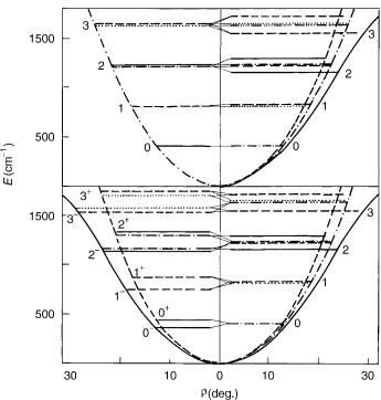
Now, let us consider a realistic case when the splitting of the potential surfaces is small, but not negligible. These potentials are drawn on the left-hand side of Figure 1, bottom (they correspond quantitatively to the A3 u state of NCN [28,29]), and on the right-hand side of both the bottom and the top part of Figure 1. Besides, the mean potential is depicted on the right-hand side, having the same form as the potential on the left-hand side of Figure 1, top, that we considered in the above discussion. All potentials are assumed to be harmonic. On the right-hand side of Figure 1 are also displayed the vibronic energy levels for the A3 u state of NCN (corresponding to the value zero of the spin quantum number).

The bottom part of Figure 1 corresponds to the ‘‘bent’’ and the upper part to the ‘‘linear’’ point of view in interpreting the R–T effect. The right-hand side of the upper part shows how the splitting of the potential surfaces affects the positions of vibronic levels; so, for example, the three u ¼ 1 levels now have different energies, and the only degeneracy that remains is that of the two components (K ¼ 2 and 2) of the jKj ¼ 2 vibronic level. The two K ¼ 0 levels differ in their symmetry with respect to reflection in the molecular plane (þ= ). The K ¼ 2 level has the energy close to that of the unperturbed vibrational level u ¼ 1; l ¼ 1. This is a general characteristic of the lowest lying level (‘‘unique’’ level [8]) for each K ¼6 0 vibronic series. The explanation is

K ¼ u þ , correspond exclusively to u, l ¼ K unperturbed levels, because the u, l ¼ K þ ¼ u þ 2 levels do not exist (remember that jlj u).

The ‘‘bent’’ point of view offers the explanation of one other aspect of the vibronic energy pattern presented. On the left-hand side of the bottom part of Figure 1 are presented the bending levels for two electronic states having the same potential surface as the components of the state considered. This situation can be looked upon as a particular case, ¼ 0, of the matrix representation (25); the coupling between the electronic states vanishes and each of them has its own bending levels with the pattern analogous to that on the left-hand side of Figure 1, top. The difference in the vibronic structure of two and a electronic state is caused by the presence of the off-diagonal elements of the matrix (25) in the latter case. However, even in electronic states the offdiagonal elements vanish for the particular case K ¼ 0 and these vibronic levels belong exclusively to one of the adiabatic electronic states. This is indicated symbolically on the right-hand side of Figure 1 by the corresponding energy level lines matching exactly one of the adiabatic potential curves. The þ= symmetry of a K ¼ 0 level is determined by the symmetry of the adiabatic state

it belongs to (þ for A1, B2, A0, for B1, A2, A00). Because for electronic states¼ 1, these levels coincide exactly with the l ¼ 1 (i.e., K ¼ 1) levels of one of the electronic species. The existence of vibrational levels not being perturbed by the vibronic coupling is of great importance for spectroscopists, because it enormously facilitates the derivation of the shape of the adiabatic potential surfaces from measured data.

All vibronic levels in spatially degenerate electronic states except K ¼ 0 species are more or less shared between both the adiabatic electronic states. The unique levels are almost equally shared between two adiabatic electronic states—their energetic position is such as if they belong to the mean adiabatic potential (Vþ þ V Þ=2. We indicate this on the right-hand side of Figure 1 by the vibronic energy lines matching exactly with the mean potential curve. The other K ¼6 0 levels belong predominantly to a particular adiabatic electronic state; this is indicated by the lines nearly matching one of the potential curves on the right-hand side of Figure 1.

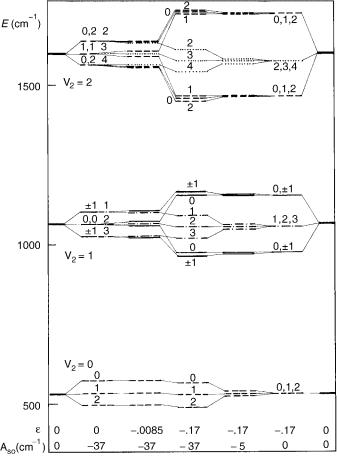
The situation in singlet electronic states of triatomic molecules with linear equilibrium geometry is presented in Figure 2. This vibronic structure can be interpreted in a completely analogous way as above for species. Note that inelectronic states there is a single unique level for K ¼ 1, but for each other K 6¼ 0 series there are two levels with a unique character.

2.Combined Vibronic and Spin–Orbit Coupling in Linear Molecules

Let us see now how the situation is changed in the presence of the spin–orbit coupling. In the central part of Figure 3 are presented the low-lying vibronic levels of the A3 u state of NCN, as obtained in recent ab initio calculations [28,29]. On the left and right edge of the figure are displayed the bending vibrational levels corresponding to the case when both the vibronic and spin– orbit coupling are absent.

Going from left to right, we show in the second column the results of calculations in which the spin–orbit constant is set to be Aso ¼ 37 cm 1 (as computed in the mentioned studies) and the vibronic coupling is neglected (e ¼ 0). The parameter e is the ‘‘Renner parameter,’’ defined for electronic states as the ratio of the (quadratic) force constants for the difference and the sum of the adiabatic bending potentials. Inspection of the secular equation (32) shows that in this case there exist three doubly degenerate effective bending potentials, involving the mean electronic energy and the contribution from the spin–orbit part of the Hamiltonian, with the energy spacing equal to jAsoj: The lowest energy ones correspond to ð¼ 1Þ, ¼ 1 and , ¼ 1; the next two to , ¼ 0 and , ¼ 0; and the highest energy pair to , ¼ 1 and, ¼ 1. Each zeroth-order vibrational level with a particular value u is now split into three levels, each one belonging to one of the effective potentials. These levels are generally degenerate, involving all possible K species with the

Figure 2. Relationship between bending vibrational structure in electronic states and vibronic structure in states. Left, top: Bending vibrational structure in a electronic state of a triatomic molecule with linear equilibrium geometry. Left, bottom: Bending vibrational structure of two electronic states with the same minimum of bending potential curves. Right: Vibronic structure of a electronic state of a molecule with linear equilibrium geometry. Solid curve: Bending potential curve for the lower lying adiabatic electronic state. Dashed curve: bending potential curve for the upper adiabatic electronic state. Dash–dotted curve: mean bending potential. Bending vibrational structure in a electronic state of a triatomic molecule with linear equilibrium geometry. Solid horizontal lines: l ¼ 0 vibrational levels for electronic states, K ¼ 0 vibronic levels for electronic state. Dashed horizontal lines: l ¼ 1 and K ¼ 1 levels. Dash–dotted lines: l ¼ 2 and K ¼ 2 levels. Dotted lines: l ¼ 3 and K ¼ 3 levels. Vibrational levels are assigned by the quantum numbers u2. The u2 and uþ2 quantum numbers at the bottom left part of the figure denote vibrational levels belonging to the lower and upper electronic state, respectively.

combinations of quantum numbers , associated with the effective potential in question. The exception are the u ¼ 0 levels, being nondegenerate (except for the jKj degeneracy).

Introduction of the vibronic coupling (e 6¼ 0) causes removal of the above degeneracy and leads to the general vibronic–spin–orbit pattern presented in the central part of Figure 3. Each vibronic level is characterized by a particular K

Figure 3. Low-energy vibronic spectrum in a 3 electronic state of a linear triatomic molecule, computed for various values of the Renner parameter e and spin–orbit constant Aso (in cm 1). The spectrum shown in the center of figure (e ¼ 0:17; Aso ¼ 37cm 1) corresponds to the A3 u state of NCN [28,29]. The zero on the energy scale represents the minimum of the potential energy surface. Solid lines: K ¼ 0 vibronic levels; dashed lines: K ¼ 1 levels; dash-dotted lines: K ¼ 2 levels; dotted lines: K ¼ 3 levels. Spin–vibronic levels are denoted by the value of the corresponding quantum number PðP ¼ K þ ; note that is in this case spin quantum number).

and P ¼ K þ quantum number (i.e., by a particular K, combination). The exception represents the K ¼ 0, P ¼ 1 levels remaining degenerate with each other. In the case when the vibronic coupling is weak compared to the spin–orbit coupling (eo Aso) the coarse structure of the spectrum is determined by the spin–orbit effects. This is illustrated in Figure 3 with the case e ¼ 0:0085

(corresponding to eo ¼ 4:5 cm 1Þ; Aso ¼ 37 cm 1; note, for example, that the u ¼ 1, K ¼ 0 levels are divided into three pairs of close-lying levels, with successive energetic separation between these pairs nearly equal to the value of the spin–orbit constant.

Now, let us consider the rising of the vibronic–spin–orbit structure from the ‘‘opposite side,’’ that is, when the vibronic interaction is dominant compared to the spin–orbit coupling (right-hand side part of Figure 3). The structure of the vibronic spectrum for the nonzero value of the Renner parameter (in the concrete case e ¼ 0:17) and Aso ¼ 0 has been disussed above (Fig. 1). The only difference is that each vibronic level is now threefold spin degenerate. When an additional weak spin–orbit interaction is added [Fig. 3, e ¼ 0:17, Aso ¼ 5 cm 1 (arbitrary choice)], the spin degeneracy of the vibronic levels is removed, but the energy pattern is quite different from that corresponding to the oposite case of strong spin–orbit and weak vibronic coupling, discussed above. The coarse structure of the spectrum is the same as in the case of no spin–orbit coupling, with the latter interaction causing a relatively small additional splitting of vibronic levels. This splitting is maximally pronounced in unique levels, where it is nearly equal to the value of Aso, and almost negligible in nonunique levels. This is a consequence of the composition of the corresponding wave functions. In the first approximation, the magnitude of the spin–orbit splitting is given by Aso hLzi, where hLzi is the mean value of the electronic angular momentum operator in the vibronic state considered. While the unique level belongs almost exclusively to a single diabatic electronic state (þ ) and thus hLzi is nearly equal to for it, the other levels belong predominantly to a particular adiabatic electronic species, or, in other words they are nearly equally shared between the diabatic states þ and with the result that hLzi is close to zero in them. Each K ¼ 0 level, being threefold spin degenerate at Aso ¼ 0, splits at nonvanishing spin–orbit coupling into two levels; the single one corresponds to ¼ 0 (i.e., K ¼ P ¼ 0), and the twofold degenerate level involvs 1 spin states. The latter vibronic states cannot be exactly classified into þ and species according to their behavior upon reflections in symmetry planes.

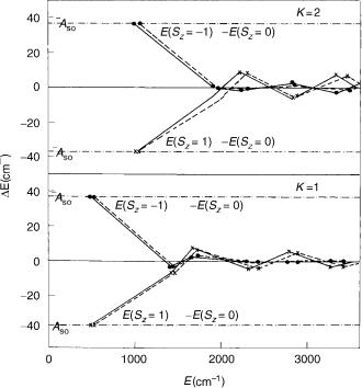
When the vibronic and spin–orbit coupling are comparably strong, as in the A3 u state of NCN (actually, although eo and Aso are in this case of the same magnitude order, the former quantity is roughly by a factor of 3 largen than the latter), the coarse structure of the part of the spectrum corresponding to a particular quantum number u is characterized by (1) a relatively large energetic separation of the unique level from its nonunique counterparts; (2) relative proximity of nonunique levels with different K values; (3) relatively large spin–orbit splitting (roughly equal to the magnitude of Aso) of the unique level; (4) an efficiently quenched spin–orbit splitting in other levels. Figure 4 presents the ab initio computed dependence of the spin–orbit splitting in K ¼ 1 and 2 levels on the

Figure 4. Spin–orbit splitting in K ¼ 1 and 2 vibronic levels of the A3 u state of NCN. Solid lines connect the results of calculations that employ ab initio computed potential curves [28]. For comparison the results obtained by employing experimentally derived potential curves (dashed lines) [30,31] are also given. Full points represent energy differences between P ¼ K 1 and P ¼ K spin levels, and crosses are differences between P ¼ K þ 1 and P ¼ K levels.

value of the bending quantum number u. It shows a ‘‘sawtooth’’ pattern, reflecting the erratic change of the vibronic mean value for the electronic angular momentum from one level to the other, typical for such systems (see also [26]).

The above results of ab initio calculation for the A3 u state of NCN (completed by those employing hypothetical values for e and Aso) correspond to the schematic presentation of the effect of combined vibronic and spin–orbit couplings onto the spectral structure of 3 states of linear triatomics, carried out by Hougen [32] and reproduced in Herzberg’s book (see Fig. 9 and accompanied discussion in [5]). A more detailed insight can be achieved by inspecting the perturbative formulae given in Appendix A.

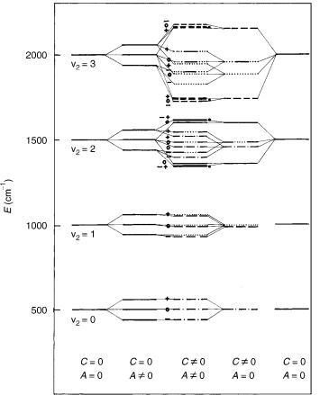
The vibronic structure of a 3 electronic state at variable strengths of the vibronic and spin–orbit coupling is presented in Figure 5. The splitting of the

Figure 5. Low-energy vibronic spectrum in a 3 electronic state of a linear triatomic molecule. The parameter c determines the magnitude of splitting of adiabatic bending potential curves, Aso is the spin–orbit coupling constant, which is assumed to be positive. The zero on the energy scale represents the minimum of the potential energy surface. ———— : K ¼ 0 vibronic levels; - - - - - - : K ¼ 1 levels; — — : K ¼ 2 levels; . . . . . . . . . :K ¼ 3 levels; — . . . — : K ¼ 4 levels; . . . — . . . : K ¼ 5 levels. Spin-vibronic levels are denoted by a minus ( ¼ 1) , zero ( ¼ 0), or plus ( ¼ þ1). Note that is in this case spin quantum number.

adiabatic bending potential curves is assumed in to be in the form Vþ V ¼ cr4. Note that in states the maximal splitting of the vibronic levels upon spin–orbit coupling (taking place in unique levels) is 2Aso. The vibronic structure of the 3 electronic state is not considered explicitly in Herzberg’s book.