Baer M., Billing G.D. (eds.) - The role of degenerate states in chemistry (Adv.Chem.Phys. special issue, Wiley, 2002)

the most usual and best studied spectroscopic problems. A great part of radicals being of crucial interest from an astrophysical/chemical point of view and/or playing as reaction intermediates an important role in various chemical processes have spatially degenerate ground states and thus exhibit the R–T effect. This circumstance determines not only the spectral features of such radicals, but also their behavior in chemical reactions.

A consequence of the continuously growing importance of such systems is the appearance of several excellent reviews devoted to this subject. A comprehensive presentation of the theoretical and experimental situation in this field up to 1974 is given by Duxbury (one of very few ‘‘R–T’’ titles up to that time) [11]. Jungen and Merer’s [8] breakthrough paper from 1976 presents various theoretical aspects of the R–T effects in triatomics, particularly the relationship between two apparently opposite, but in fact equivalent, points of views (electrostatic interaction within a degenerate electron state—Coriolis interaction between two separate states). A critical exposure of different models for handling the R–T effect is given by Brown and Jørgensen [12]: It is recommended to everyone who is interested in this subject, particularly to those who really want to understand it completely, although we find this article the most difficult of all mentioned so far. Ko¨ppel et al. [13] and Ko¨ppel and Domcke [14] present the R–T effect as a particular case of a general multistate and multimode problem. Their models are deliberately so simplified that they enable clear insight into the mechanisms being otherwise obscured. Recently, Brown [3] has given a very clear presentation of the effective Hamiltonian approaches used in experimental investigations of the R–T effect, and a very detailed description of a highly sophisticated theoretical approach has been presented by Jensen et al. [2]. Furthermore, the R–T effect is described in detail in several standard textbooks, for example, by Herzberg [5]. and Bunker and Jensen [15]. Finally, let us mention the reviews by the present authors, which refer to early ab initio studies on triatomic [16,17] and tetraatomic [18] species.

Taking into account that there already exists such a comprehensive literature on the R–T effect, the question naturally arises: Is there a need to write a new review devoted to this subject? Is it, for example, possible to add anything relevant to the review by Brown and Jørgensen [12], to present the matter more clearly than Jungen and Merer [8], or more elegantly than Ko¨ppel et al. [13,14]? However, most of the reviews mentioned above are based on the results of their authors and reflect the authors’ particular point of view. We feel that a comparison of different approaches is still missing. This is what we try to do in this chapter. Emphasis will be put on results of ab initio methods, but a discussion of approaches based on the use of experimentally derived parameters (potential energy surfaces, equilibrium geometries, etc.) will also be included, because these approaches can be employed equally well (and several of them have been) if the parameters are generated in ab initio calculations.

III.TRIATOMIC MOLECULES

A.Theoretical Treatment

Let us start with a description of the bending vibrations in singlet electronic states of linear triatomic molecules. Already, this simple sentence reflects some of the difficulties with which one is confronted by handling the present subject: The adjective ‘‘linear’’ looks pleonastic in connection with ‘‘ states,’’ because only linear molecules can have electronic states. On the other hand, we speak about bending of molecules in states. The rigorous meaning of the mentioned sentence is that we consider the bending vibrations of a molecule with linear equilibrium geometry, at which it is in a electronic state; upon bending, the state of the molecule transforms into one of the species classified according to the irreducible representations of the lower symmetry point group corresponding to the bent nuclear arrangement. In this chapter we shall frequently be forced, in order to save time and space, to use similar phrases that may not be strictly correct from a scientific and/or linguistic point of view. Returning now to our problem, we assume the model Hamiltonian in the form

H ¼ He þ Tb þ Trz ð1Þ

where He is the electronic Hamiltonian involving the kinetic energy of electrons, their mutual interaction, and the interaction of the electrons with the nuclei. Furthermore, we assume that He also includes the nuclear repulsion term. The term Tb is the kinetic energy operator for the bending vibrations of nuclei. It involves the derivatives of the coordinate r, defined as a supplement of the bond angle (in radian) and can be written in the form

[Atomic units (me 1; qe 1; h 1) are used throughout this chapter.] The coefficients T1, T2, and T0 are assumed to be in general analytical functions of the bending coordinate r. The term Trz represent the operator describing the rotation of the molecule around the (principal) axis z corresponding to the smallest moment inertia—this axis coincides at the linear nuclear arrangement with the molecular axis. Now Trz can be written in the form

where A ¼ 1=ð2Izz) is the rotational constant and Rz is the z component of the angular momentum of the nuclei. The operator Rz is defined as

where f represents the angle between the instantaneous molecular plane and the space-fixed plane with which it has a common z axis. The model Hamiltonian [Eq. (1)] commutes with Rz and thus the quantum number l corresponding to the latter operator is a good quantum number. It is an integer as any quantum number for projection of a spatial angular momentum. The literature often refers to l as the absolute value of the eigenvalue Rz; we shall consider it here as a signed quantity.

Explicit forms of the coefficients Ti and A depend on the coordinate system employed, the level of approximation applied, and so on. They can be chosen, for example, such that a part of the coupling with other degrees of freedom (typically stretching vibrations) is accounted for. In the space-fixed coordinate system at the infinitesimal bending vibrations, Tb þ Trz reduces to the kinetic energy operator of a two-dimensional (2D) isotropic harmonic oscillator,

where m is the corresponding reduced mass. The Hamiltonian [Eq. (1)] does not involve the terms describing the stretching vibrations and the end-over-end rotations. It is supposed that these degrees of freedom can be separated from those considered here.

The wave function corresponding to the Hamiltonian [Eq. (1)] can be assumed in the form

where represents the electronic wave function and f is the r-dependent part of the nuclear function. Here m is the running index numbering vibrational states corresponding to a particular l state. After integrating over the electronic coordinates and f, the Schro¨dinger equation corresponding to the Hamiltonian

(1) becomes

VðrÞ represents the potential energy surface for bending vibrations obtained by solving the electronic Schro¨dinger equation in the BO approximation; it is two dimensional, but invariant with respect to the coordinate f. In the harmonic approximation, the potential energy function V(r) is represented by 1/2 k r2, where k is the force constant for the bending vibrations, and the kinetic energy operator is then given by Eq. (5) (with q2=qf2 replaced by l2). The solutions

the harmonic bending frequency, o ¼ pðk=mÞ (to simplify the orthography we

use for the bending frequency symbol o instead of more usual o2). The corresponding wave functions are

given u, the quantum number l takes values u, u þ 2, . . ., 1 or 0, . . ., u 2, u. Since the bending energy (in the harmonic approximation) depends only on the quantum number u, a vibrational level is thus u þ 1 times degenerate.

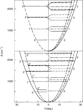
In the harmonic approximation, the bending vibrational energy scheme for a singlet electronic state corresponds to the upper part of the left-hand side of Figure 1 (given below in Section III.B). Anharmonicity of the bending potential would cause splitting of the levels with the same quantum number u but different l; while the latter of them remains a good quantum number, because the axial symmetry of the problem is also preserved when the anharmonicity is introduced, the former becomes an approximate good quantum number. In the framework of this model ( electronic states, neglected effects of end-over-end rotations, etc.) the bending energy does not depend on the sign of l; this is a reason for the above mentioned widely used convention that assumes l to be a nonnegative integer and for representing the levels corresponding to the same absolute value of l by a single line in Figure 1. Remember, however, that every jlj 6¼ 0 level is twofold degenerate.

Let us see now how the situation is changed if the molecule is a spatially degenerate electronic state. This state has two components that are at linear molecular geometry exactly degenerate with each other. Upon bending, however, the symmetry of the nuclear framework is reduced, consequently having a splitting of the potential surfaces for these component states. At least at small deviation from linearity these two electronic surfaces lie energetically close to each other and the ansatz [Eq. (6)], which assumes the vibronic wave function as a product of a single electronic species with the corresponding vibrational function, ceases to be reliable. Instead, we have to employ the wave

where c1 and c1 are electronic (at the moment not specified more precisely) species and f1, f2 are function of the nuclear coordinates.

Now, we have besides the vibrational, the electronic angular momentum; the latter is characterized by the quantum number corresponding to the magnitude of its projection along the molecular axis, Lz. Here we shall consider as a unsigned quantity, that is, for each 6¼ 0 state there will be two possible projections of the electronic angular momentum, one corresponding to and the other to . The operator Lz can be written in the form

where y is the coordinate describing collective rotations of the electrons around the z axis. This one-electron approximation was severely criticized by Brown and Jørgensen [12]. Note that, although it will be used in this chapter in several instances in order to achieve a simple presentation of some results, it will never be necessary to apply explicitly expression (11). In handling the R–T effect, one actually needs the (electronic) matrix elements of the operator Lz, which can be derived without assuming that the operator has the form (11). Trying, however, to reconcile the ansatz (11) with justified critics of the authors of [13], we can interpret y as a coordinate (in general without obvious physical meaning) conjugate to the electronic angular momentum Lz.

The presence of two angular momenta has as a consequence that only their sum, representing the total angular momentum in the case considered, necessary commutes with the Hamiltonian of the system. Thus only the quantum number K, associated with the sum, Nz, of Rz and Lz,

must be a good quantum number, not necessarily l and . It can be easily shown that this is really the case, that is, that l and are generally not even approximately good quantum numbers. The operator for rotation of the nuclei around the z axis can now be written as

Now, we add to (1) the operator describing the spin–orbit (SO) coupling, so that our model Hamiltonian becomes

We shall consider only the leading part of the spin–orbit operator assumed in the phenomenological form

where Aso is the ‘‘spin–orbit constant’’ and Sz the z component of the electronic spin operator. The Hamiltonian [Eq. (15)] commutes with the z component of the spin operator, Sz, and of the total angular momentum, Jz ¼ Nz þ Sz. Consequently, the corresponding quantum numbers (we choose this symbol in spite of the fact that it is also used to denote ¼ 0 electronic states and K ¼ 0 vibronic species) and P ¼ K þ are good quantum numbers. In the framework of this model, such also remains the quantum number K. This is not rigorously the case in treatments of the R–T effect at higher levels of sophistication. It can be stated, however, that K is one of the best among ‘‘bad’’ quantum numbers used in molecular spectroscopy. Thus the handling of the R–T effect in the framework of this model can be carried out within a particular K and P (i.e., ) subspace separately. In this chapter, we consider K, , and P to be signed; since the vibronic (vibration–electronic) levels with jKj ¼6 0 (and jPj ¼6 0) are always doubly degenerate in the framework of this model [one state corresponding to K ¼ þjKj and the other to K ¼ jKj (and analogously for P ¼ þjPj and P ¼ jPj)], we shall deal, as a rule with nonnegative values for K and P only.

Until now we have implicitly assumed that our problem is formulated in a space-fixed coordinate system. However, electronic wave functions are naturally expressed in the system bound to the molecule; otherwise they generally also depend on the rotational coordinate f. (This is not the case for electronic states, for which the wave functions are invariant with respect to f.) The eigenfunctions of the electronic Hamiltonian, cþe and ce , computed in the framework of the BO approximation (‘‘adiabatic’’ electronic wave functions) for two electronic states into which a spatially degenerate state of linear molecule splits upon bending,

are labeled by a plus or minus according to their behavior with respect to reflection in the molecular plane. The species cþ (of A1 or B2 symmetry in the C2v point group, and of A0 in Cs) is invariant upon this reflections, and c (belonging to B1 or A2 irreducible representation in the C2v point group, and to A00 in Cs) changes sign. For the sake of convenience, we assume throughout this chapter that the phase factor in c is i. Both Vþ and V are the corresponding adiabatic potentials. Therefore, these wave functions rotate together with the molecular plane. It is thus convenient (although not necessary) to formulate the complete problem in the coordinate system rotating with the molecule in the way

that a plane of this frame (we chose it to be xz) coincides with the instantaneous molecular plane at bent nuclear arrangements. We introduce the coordinate transformation

a is therefore the electronic azimuthal coordinate with respect to the molecular plane. It is easy to prove that the nuclear, electronic, and total (excluding spin) angular momenta defined with respect to the molecule-bound frame are

Apparently, the most natural choice for the electronic basis functions consist of the adiabatic functions cþe and ce defined in the molecule-bound frame. By making use of the assumption that K is a good quantum number, we can write the complete vibronic basis in the form

The electronic functions are assumed to be eigenfunctions of the spin operator and are thus assigned by the spin quantum number . Their dependence on a, indicated in Eq. (20), should not be taken too seriously; it should just remind us that the functions are defined in the molecule-bound frame, that is, that they do not depend on the nuclear rotational coordinate f. The bending functions f þ and f , corresponding to the electronic species cþ and c , respectively, are additionally labeled by K and a running index n. The electronic Hamiltonian and the operator Tb are diagonal in the adiabatic electronic basis. The operator Rz couples the functions cþ and c with each other. Although only the nuclear angular momentum Rz appears explicitly in the model Hamiltonian [Eq. (15)], the electronic angular momentum creeps into its matrix representation as a consequence of the first of relations (19) and the form of the basis functions. The adiabatic electronic functions are, namely, not the eigenfunctions of Lz. Let us denote the electronic matrix elements of the operators Lz and L2z by

The remaining combinations vanish for symmetry reasons [the operator Lz transforms according to B1 (A00) irreducible representation]. The nonvanishing of the off-diagonal matrix element Bþ is responsible for the coupling of the adiabatic electronic states.

electronic states cþ and c can be carried out straightforwardly. In order to have expressions more suitable for discussing the spectroscopic aspects of this problem, we now replace the matrix elements B and C by their asymptotic values (23) and the kinetic energy operator by its small-amplitude counterpart (5) [note, however, that the asymptotic forms of the electronic wave functions, Eq. (25), cannot be employed for calculation of the matrix elements of the electronic operator He]:

The basis consisting of the adiabatic electronic functions (we shall call it ‘‘bent basis’’) has a serious drawback: It leads to appearance of the off-diagonal elements that tend to infinity when the molecule reaches linear geometry (i.e., r ! 0). Thus it is convenient to introduce new electronic basis functions by the transformation

We write them as c ðyÞ to stress that now we use the space-fixed coordinate frame. We shall call this basis ‘‘diabatic,’’ because the functions (26) are not the eigenfunction of the electronic Hamiltonian. The matrix elements of He are

We shall call this basis also ‘‘linear’’ because in the one-electron approximation at r ! 0 the functions (26) become

that is, they reduce to the functions describing free rotation of electrons around the molecular axis. These asymptotic forms of the basis functions may be used in