Laser-Tissue Interactions Fundamentals and Applications - Markolf H. Niemz

68 3. Interaction Mechanisms

3.2.1 Heat Generation

By means of the two-step process as described above, heat is generated inside the tissue during laser exposure. Deposition of heat in tissue is due only to light that is absorbed in the tissue. For a light flux in the z-direction in a nonscattering medium, the local heat deposition per unit area and time in a thickness Δz is given by

Thus, the heat source S(r,z,t) inside the exposed tissue is a function of the absorption coe cient α and the local intensity I(r,z,t). Since α is strongly wavelength-dependent, the same applies for S. If phase transitions (vaporization, melting) or tissue alterations (coagulation, carbonization) do not occur, an alteration in heat content dQ induces a linear change in temperature dT according to a basic law of thermodynamics

where m is the tissue mass, and c is the specific heat capacity expressed in units of kJ kg−1 K−1. According to Takata et al. (1977), for most tissues, a good approximation is given by

where is the tissue density expressed in units of kg/m3, and w is its water content expressed in units of kg/m3. In the case of water, i.e. w = , the last relation reduces to

3.2.2 Heat Transport

Within a closed physical system, the relationship between temperature and heat content is described by (3.4). In real laser–tissue interactions, however, there are losses of heat to be taken into account, as well. They are based on either heat conduction, heat convection, or heat radiation. Usually, the latter two can be neglected for most types of laser applications. One typical example

of heat convection in tissue is heat transfer due to blood flow. The perfusion rates of some human organs are summarized in Table 3.4. Due to the low perfusivity of most tissues, however, heat convection is negligible in a first approximation. Only during long exposures and in special cases such as laserinduced interstitial thermotherapy (LITT) does it play a significant role and should be considered by adding a negative heat loss Sloss to the source term S. Heat radiation is described by the Stefan–Boltzmann law which states that the radiated power is related to the fourth power of temperature. Due to the moderate temperatures achieved in most laser–tissue interactions, heat radiation can thus often be neglected.

Table 3.4. Blood perfusion rates of some selected human organs. Data according to Svaasand (1985)

Heat conduction, though, is a considerable heat loss term and is the primary mechanism by which heat is transferred to unexposed tissue structures. The heat flow jQ is proportional to the temperature gradient according to the general di usion equation2

Herein, the constant k is called heat conductivity and is expressed in units of W m−1 K−1. According to Takata et al. (1977), k can be approximated by

In the case of water, i.e. w = , the last relation reduces to

The dynamics of the temperature behavior of a certain tissue type can also be expressed by a combination of the two parameters k and c. It is called temperature conductivity and is defined by

2This equation is the analog to the electrodynamic equation j = −σ φ, where j is the electric current density, σ is the electric conductivity, and φ is the electric potential.

The value of κ is approximately the same for liquid water and most tissues

– about 1.4 × 10−7 m2/s according to Boulnois (1986) – since a decrease in heat conductivity due to a lower water content is usually compensated by a parallel decrease in heat capacity.

With these mathematical prerequesites, we are able to derive the general heat conduction equation. Our starting point is the equation of continuity which states that the temporal change in heat content per unit volume3, q˙, is determined by the divergence of the heat flow jQ:

The other important basic equation is the di usion equation, i.e. (3.5). Its combination with (3.8) yields

equation with the temperature conductivity as defined by (3.6). With an additional heat source S like the absorption of laser radiation, (3.8) and (3.9) turn into the inhomogeneous equations

Next, we want to solve the homogeneous part of the heat conduction equation, i.e. (3.9). It describes the decrease in temperature after laser exposure due to heat di usion. In cylindrical coordinates, (3.9) can be expressed by

with the general solution

3Note that q in (3.7) is expressed in units of J/cm3, while Q is in units of J. We thus obtain according to Gauss’ theorem: dV divjQ = df jQ = −Q˙ .

where T0 is the initial temperature, and χ0 is an integration constant. The proof is straightforward. We simply assume that (3.13) represents a correct solution to (3.12) and find

The solution to the inhomogeneous heat conduction equation, (3.11) strongly depends on the temporal and spatial dependences of S(r,z,t). Usually, it is numerically evaluated assuming appropriate initial value and boundary conditions. Nevertheless, an analytical solution can be derived if the heat source function S(r,z,t) is approximated by a delta-function

S(r,z,t) = S0 δ(r −r0) δ(z −z0) δ(t −t0) .

For the sake of simplicity, we assume that the heat conduction parameters are isotropic4. Thus,

S(z,t) = S0 δ(z −z0) δ(t −t0) .

In this case, the solution can be expressed by a one-dimensional Green’s function which is given by

By means of this function, the general solution for a spatially and temporally changing irradiation is determined by

4A valuable theoretical approach to the three-dimensional and time-dependent problem is found in the paper by Halldorsson and Langerholc (1978).

The term “penetration depth” originates from the argument of the exponential function in (3.14), since (3.16) turns into

ztherm2 (t) = 1 .

4κt

Thus, ztherm(t) is the distance in which the temperature has decreased to 1/e of its peak value. In Table 3.5, the relationship expressed by (3.16) is evaluated for water (κ = 1.4×10−7 m2/s). We keep in mind that heat di uses in water to approximately 0.7μm within 1μs.

Table 3.5. Thermal penetration depths of water

For thermal decomposition of tissues, it is important to adjust the duration of the laser pulse in order to minimize thermal damage to adjacent structures. By this means, the least possible necrosis is obtained. The scaling parameter for this time-dependent problem is the so-called thermal relaxation time according to Hayes and Wolbarsht (1968) and Wolbarsht (1971). It is obtained by equating the optical penetration depth L as defined by (2.16) to

where τtherm is the thermal relaxation time. One might argue the significance of τtherm, because it is a theoretically constructed parameter. During thermal decomposition, however, τtherm becomes very important, since it measures the thermal susceptibility of the tissue. This shall be explained by the following consideration: for laser pulse durations τ < τtherm, heat does not even di use to the distance given by the optical penetration depth L. Hence, thermal damage of nondecomposed tissue is neglible. For τ > τtherm, heat can di use to a multiple of the optical penetration depth, i.e. thermal damage of tissue adjacent to the decomposed volume is possible.

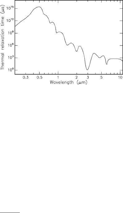
Fig. 3.18. Thermal relaxation times of water

Because of (3.17), the wavelength-dependence of L2 is transferred to τtherm. In Fig. 3.18, thermal relaxation times of water are shown as calculated from Fig. 3.14 and (3.17). We find that the shortest thermal relaxation time of approximately 1μs occurs at the absorption peak of water near 3μm. We may thus conclude that laser pulse durations τ < 1μs are usually5 not associated with thermal damage. This statement is also referred to as the “1μs rule”.

–Case I: τ <1μs. For nanoor picosecond pulses, heat di usion during the laser pulse is negligible. If, in addition, we make the simplifying assumption that the intensity is constant during the laser pulse, we obtain from (3.3) that

S = αI0 .

For a quantitative relationship T(t) at the tissue surface (r = z = 0), we may write

5Laser pulses shorter than 1μs can also lead to thermal e ects if they are applied at a high repetition rate as discussed later in this section.

74 3. Interaction Mechanisms

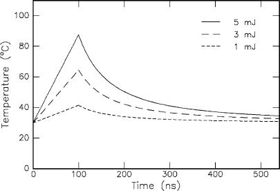
In Fig. 3.19, the temporal evolution of temperature in the pigment epithelium of the retina is shown according to (3.18). By neglecting heat di usion during the short laser pulse, the temperature first increases linearly with respect to time. After the laser pulse, i.e. t > τ, it decreases according to t−3/2 as determined by the solution to the homogeneous heat conduction equation. The thermally damaged zone is shorter than the optical absorption length. Thus, thermal damage to adjacent tissue can be kept small if a wavelength is selected that is strongly absorbed by the tissue. In the case of tissues with a high water content, Er:YAG and Er:YSGG lasers are potential candidates for this task. However, only a few groups like Andreeva et al. (1986), Eichler et al. (1992), and Pelz et al. (1994) have reported on mode locking of these lasers. But their operation is not yet stable enough for clinical applications. Alternatives might soon arise due to recent advances in the development of tunable IR lasers such as the optical parametric oscillator (OPO) and the free electron laser (FEL).

Fig. 3.19. Temporal evolution of temperature in the pigment epithelium of the retina during and after exposure to a short laser pulse (τ = 100ns, beam diameter: 2mm, pulse energy: as labeled, T0 = 30◦C, α = 1587cm−1, = 1.35g cm−3, and c = 2.55J g−1 K−1). Tissue parameters according to Hayes and Wolbarsht (1968) and Weinberg et al. (1984)

–Case II: τ > 1μs. For pulse durations during which heat di usion is considerable, the thermally damaged zone is significantly broadened. In this case, the solution to the inhomogeneous heat conduction equation cannot be given analytically but must be derived numerically, for instance by using the methods of finite di erences and recursion algorithms. This procedure

becomes necessary because heat di usion during the laser pulse can no longer be neglected. Thus, for this period of time, temperature does not linearly increase as assumed in (3.18) and Fig. 3.19. Detailed simulations were performed by Weinberg et al. (1984) and Roggan and M¨uller (1993). One example is found in Fig. 3.24 during the discussion of laser-induced interstitial thermotherapy.

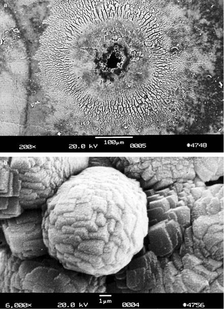
A high repetition rate νrep of the laser pulses can evoke an additional increase in temperature if the rate of heat transport is less than the rate of heat generation. The dependence of temperature on repetition rate of the laser pulses was modeled by van Gemert and Welch (1989). The significance of the repetition rate becomes evident when looking at Figs. 3.20a–b. In this case, 1000 pulses from a picosecond Nd:YLF laser were focused on the same spot of a human tooth at a repetition rate of 1kHz. Although, usually such short pulses do not evoke any thermal e ect as discussed above, radial cracking and melting obviously occurred at the surface of the tooth. In particular, the enlargement shown in Fig. 3.20b demonstrates that the chemical compounds of the tooth had melted and recrystallized in a cubic structure. Thus, the temperature achieved must have reached a few hundred ◦C due to insu cient heat transport.

In order to get a basic feeling for typical laser parameters, the following very simple calculations might be very useful. We assume that a pulse energy of 3μJ is absorbed within a tissue volume of 1000μm3 which contains 80% water. The amount of water in the specified volume is equal to 8×10−10 cm−3 or 8×10−10 g, respectively. There are now three steps to be taken into account when aiming for a rough approximation of the final temperature. First, energy is needed to heat the tissue up to 100◦C. Second, energy is transferred to vaporization heat. And third, the remaining energy leads to a further increase in temperature of the water vapor.

–Step 1: 37◦C −→ 100◦C (assumed body temperature: 37◦C) Q1 = mcΔT = 8×10−10 g 4.3 kgkJ◦C 63◦C = 2.2×10−7 J.

–Step 2: Vaporization at 100◦C

Thus, the resulting temperature is approximately 385◦C.

3.2.3 Heat E ects

The model developed above usually predicts the spatial and temporal distribution of temperature inside tissue very well if an appropriate initial value and boundary conditions are chosen. This, however, is not always an easy task. In general, though, approximate values of achievable temperatures can often be estimated. Therefore, the last topic in our model of thermal interaction deals with biological e ects related to di erent temperatures inside the tissue. As already stated at the beginning of this section, these can be manifold, depending on the type of tissue and laser parameters chosen. The most important and significant tissue alterations will be reviewed here.

Assuming a body temperature of 37◦C, no measurable e ects are observed for the next 5◦C above this. The first mechanism by which tissue is thermally a ected can be attributed to conformational changes of molecules. These e ects, accompanied by bond destruction and membrane alterations, are summarized in the single term hyperthermia ranging from approximately 42–50◦C. If such a hyperthermia lasts for several minutes, a significant percentage of the tissue will already undergo necrosis as described below by Arrhenius’ equation. Beyond 50◦C, a measurable reduction in enzyme activity is observed, resulting in reduced energy transfer within the cell and immobility of the cell. Furthermore, certain repair mechanisms of the cell are disabled. Thereby, the fraction of surviving cells is further reduced.

At 60◦C, denaturation of proteins and collagen occurs which leads to coagulation of tissue and necrosis of cells. The corresponding macroscopic response is visible paling of the tissue. Several treatment techniques such as laser-induced interstitial thermotherapy (LITT) aim at temperatures just above 60◦C. At even higher temperatures (> 80◦C), the membrane permeability is drastically increased, thereby destroying the otherwise maintained equilibrium of chemical concentrations.

At 100◦C, water molecules contained in most tissues start to vaporize. The large vaporization heat of water (2253kJ/kg) is advantageous, since the vapor generated carries away excess heat and helps to prevent any further increase in the temperature of adjacent tissue. Due to the large increase in volume during this phase transition, gas bubbles are formed inducing mechanical ruptures and thermal decomposition of tissue fragments.

Only if all water molecules have been vaporized, and laser exposure is still continuing, does the increase in temperature proceed. At temperatures exceeding 100◦C, carbonization takes place which is observable by the blackening of adjacent tissue and the escape of smoke. To avoid carbonization, the tissue is usually cooled with either water or gas. Finally, beyond 300◦C, melting can occur, depending on the target material.

All these steps are summarized in Table 3.6, where the local temperature and the associated tissue e ects are listed. For illustrating photographs, the reader is referred to Figs. 3.10–3.13 and Fig. 3.20.