

Laser-Tissue Interactions Fundamentals and Applications - Markolf H. Niemz
.pdf18 2. Light and Matter
When comparing Figs. 2.4 and 2.5, we find that the absorption spectra of the aortic wall and hemoglobin are quite similar. This observation can be explained by the fact that hemoglobin – as already previously stated – is predominant in vascularized tissue. Thus, it becomes evident that the same absorption peaks must be present in both spectra. Since the green and yellow wavelengths of krypton ion lasers at 531nm and 568nm, respectively, almost perfectly match the absorption peaks of hemoglobin, these lasers can be used for the coagulation of blood and blood vessels. For certain clinical applications, dye lasers may be an alternative choice, since their tunability can be advantageously used to match particular absorption bands of specific proteins and pigments.
Not only the absorption of biological tissue, though, is important for medical laser surgery. In certain laser applications, e.g. sclerostomies, special dyes and inks are frequently applied prior to laser exposure. By this means, the original absorption coe cient of the specific tissue is increased, leading to a higher e ciency of the laser treatment. Moreover, adjacent tissue is less damaged due to the enhanced absorption. For further details on sclerostomy, the reader is referred to Sect. 4.1.
In Table 2.2, the e ects of some selected dyes on the damage threshold are demonstrated in the case of scleral tissue. The dyes were applied to the sclera by means of electrophoresis, i.e. an electric current was used to direct the dye into the tissue. Afterwards, the samples were exposed to picosecond pulses from a Nd:YLF laser to achieve optical breakdown (see Sect. 3.4). The absolute and relative threshold values of pulse energy are listed for each dye. Obviously, the threshold for the occurrence of optical breakdown can be decreased by a factor of two when choosing the correct dye. Other dyes evoked only a slight decrease in threshold or no e ect at all. In general, the application of dyes should be handled very carefully, since some of them might induce toxic side e ects.
Table 2.2. E ect of selected dyes and inks on damage threshold of scleral tissue. Damage was induced by a Nd:YLF laser (pulse duration: 30ps, focal spot size: 30μm). Unpublished data
Dye |
Damage threshold (μJ) |
Relative threshold |
|
|
|
None |
87 |
100% |
Erythrosine |
87 |
100% |
Nigrosine |
87 |
100% |
Reactive black |
82 |
94% |
Brilliant black |
81 |
93% |
Amido black |
75 |
86% |
Methylene blue |
62 |
71% |
Tatrazine |
62 |
71% |
Bismarck brown |
56 |
64% |
India ink |
48 |
55% |
|
|
|
2.3 Scattering |
19 |
2.3 Scattering
When elastically bound charged particles are exposed to electromagnetic waves, the particles are set into motion by the electric field. If the frequency of the wave equals the natural frequency of free vibrations of a particle, resonance occurs being accompanied by a considerable amount of absorption. Scattering, on the other hand, takes place at frequencies not corresponding to those natural frequencies of particles. The resulting oscillation is determined by forced vibration. In general, this vibration will have the same frequency and direction as that of the electric force in the incident wave. Its amplitude, however, is much smaller than in the case of resonance. Also, the phase of the forced vibration di ers from the incident wave, causing photons to slow down when penetrating into a denser medium. Hence, scattering can be regarded as the basic origin of dispersion.
Elastic and inelastic scattering are distinguished, depending on whether part of the incident photon energy is converted during the process of scattering. In the following paragraphs, we will first consider elastic scattering, where incident and scattered photons have the same energy. A special kind of elastic scattering is Rayleigh scattering. Its only restriction is that the scattering particles be smaller than the wavelength of incident radiation. In particular, we will find a relationship between scattered intensity and index of refraction, and that scattering is inversely proportional to the fourth power of wavelength. The latter statement is also known as Rayleigh’s law and shall be derived in the following paragraphs.
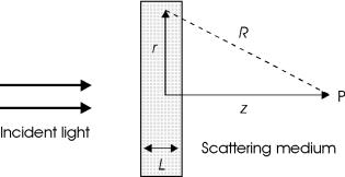
Fig. 2.6. Geometry of Rayleigh scattering
In Fig. 2.6, a simple geometry of Rayleigh scattering is shown. A plane electromagnetic wave is incident on a thin scattering medium with a total thickness L. At a particular time, the electric field of the incident wave can be expressed by
E(z) = E0 exp(ikz) ,

20 2. Light and Matter
where E0 is the amplitude of the incident electric field, k is the amount of the propagation vector, and z denotes the optical axis. In a first approximation, we assume that the wave reaching some point P on the optical axis will essentially be the original wave, plus a small contribution due to scattering. The loss in intensity due to scattering is described by a similar relation as absorption, i.e.
I(z) = I0 exp(−αsz) , |
(2.17) |
where αs is the scattering coe cient. Di erentiation of (2.17) with respect to z leads to
dI = −αsI dz .
The intensity scattered by a thin medium of a thickness L as shown in Fig. 2.6 is thus proportional to αs and L:
Is αsL . |
(2.18) |
Let us now assume that there are NL atoms per unit area of the scattering medium. Herein, the parameter N shall denote the density of scattering atoms. Then, the intensity scattered by one of these atoms can be described by the relation
I1 αNLsL = αNs .
Thus, the amplitude of the corresponding electric field is
E1 |
|
|
|
Ns |
. |
|
|
|
|
α |
|
Due to the interference of all scattered waves, the total scattered amplitude can be expressed by
Es NL |
|
|
αs |
|
|
|
|
|
= L αsN . |
||||||
|
N |
||||||
|
|
|
|
||||
The complex amplitude at a distance z on the optical axis is obtained by adding the amplitudes of all scattered spherical waves to the amplitude of the incident plane wave, i.e.
|
|
|
|
∞ |
kR |
|
|
|
eikz + L |
|
|
|
ei |
2πr dr , |
(2.19) |
E(z) = E0 |
αsN |
|
|||||
|
R |
||||||
|
|
0 |
|
|
|
||
with R2 = z2 + r2 .
At a given z, we thus obtain r dr = R dR ,
|
|
|
2.3 Scattering |
21 |
which reduces (2.19) to |
|
|
|
|
E(z) = E0 |
eikz + L |
|
2π ∞ eikR dR . |
|
αsN |
(2.20) |
|||
|
|
|
z |
|
Since wave trains always have a finite length, scattering from R → ∞ can be neglected. Hence, (2.20) turns into
|
|
|
|||
|
|
|
π |
|
|
E(z) = E0 eikz −L αsN |
2 |
eikz |
, |
||
ik |
|||||
and when inserting the wavelength λ = 2π/k
E(z) = E0 |
eikz |
1 + iλL |
|
. |
(2.21) |
αsN |
|||||
|
|
|
|
|
|
According to our assumption, the contribution of scattering – i.e. the second term in parentheses in (2.21) – is small compared to the first. Hence, they can be regarded as the first two terms of an expansion of
E(z) = E0 exp |
i |
kz + λL |
|
. |
|
αsN |
|||||
|
|
|
|
√ |
|
Therefore, the phase of the incident wave is altered by the amount λL αsN |
|||||
due to scattering. This value must be equal to the well-known expression of phase retardation given by
Δφ = 2λπ (n −1)L ,
which occurs when light enters from free space into a medium with refractive index n. Hence,
λL αsN = 2λπ(n −1)L , |
|
|
|
λ2 |
|
n −1 = |
2π αsN . |
(2.22) |
From (2.18) and (2.22), we finally obtain Rayleigh’s law of scattering when neglecting the wavelength-dependence of n, i.e.
Is |
1 |
. |
(2.23) |
4 |
|||
|
λ |
|
|
If the scattering angle θ is taken into account, a more detailed analysis yields
Is(θ) |
1 + cos2(θ) |
, |
(2.24) |
|
λ4 |
||||
|
|
|
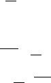
where θ = 0 denotes forward scattering. Rayleigh’s law is illustrated in Fig. 2.7. Within the visible spectrum, scattering is already significantly reduced when comparing blue and red light.
22 2. Light and Matter
Fig. 2.7. Rayleigh’s law of scattering for near UV, visible, and near IR light
Rayleigh scattering is elastic scattering, i.e. scattered light has the same values of k and λ as incident light. One important type of inelastic scattering is known as Brillouin scattering. It arises from acoustic waves propagating through a medium, thereby inducing inhomogeneities of the refractive index. Brillouin scattering of light to higher (or lower) frequencies occurs, because scattering particles are moving toward (or away from) the light source. It can thus be regarded as an optical Doppler e ect in which the frequency of photons is shifted up or down. In laser–tissue interactions, Brillouin scattering becomes significant only during the generation of shock waves as will be discussed in Sect. 3.5.
In our derivation of Rayleigh’s law, absorption has been neglected. Therefore, (2.22)–(2.24) are valid only for wavelengths far away from any absorption bands. Simultaneous absorption and scattering will be discussed in Sect. 2.4. Moreover, we did not take the spatial extent of scattering particles into account. If this extent becomes comparable to the wavelength of the incident radiation such as in blood cells, Rayleigh scattering no longer applies and another type of scattering called Mie scattering occurs. The theory of Mie scattering is rather complex and shall thus not be repeated here. However, it is emphasized that Mie scattering and Rayleigh scattering di er in two important respects. First, Mie scattering shows a weaker dependence on wavelength ( λ−x with 0.4 ≤ x ≤ 0.5) compared to Rayleigh scattering ( λ−4). Second, Mie scattering preferably takes place in the forward direction, whereas Rayleigh scattering is proportional to 1 + cos2(θ) according to (2.24), i.e. forward and backward scattered intensities are the same.
2.3 Scattering |
23 |
In most biological tissues, it was found by Wilson and Adam (1983), Jacques et al. (1987b), and Parsa et al. (1989) that photons are preferably scattered in the forward direction. This phenomenon cannot be explained by Rayleigh scattering. On the other hand, the observed wavelength-dependence is somewhat stronger than predicted by Mie scattering. Thus, neither Rayleigh scattering nor Mie scattering completely describe scattering in tissues. Therefore, it is very convenient to define a probability function p(θ) of a photon to be scattered by an angle θ which can be fitted to experimental data. If p(θ) does not depend on θ, we speak of isotropic scattering. Otherwise, anisotropic scattering occurs.
A measure of the anisotropy of scattering is given by the coe cient of anisotropy g, where g = 1 denotes purely forward scattering, g = −1 purely backward scattering, and g = 0 isotropic scattering. In polar coordinates, the coe cient g is defined by
g = |
4π p(θ) cosθ dω |
, |
(2.25) |
|
4π p(θ) dω |
|
|
where p(θ) is a probability function and dω = sinθdθdφ is the elementary solid angle. By definition, the coe cient of anisotropy g represents the average value of the cosine of the scattering angle θ. As a good approximation, it can be assumed that g ranges from 0.7 to 0.99 for most biological tissues. Hence, the corresponding scattering angles are most frequently between 8◦ and 45◦. The important term in (2.25) is the probability function p(θ). It is also called the phase function and is usually normalized by
1 |
|
p(θ) dω = 1 . |
(2.26) |
4π |
|||
|
4π |
|
|
Several theoretical phase functions p(θ) have been proposed and are known as Henyey–Greenstein, Rayleigh–Gans, δ–Eddington, and Reynolds functions2. Among these, the first is best in accordance with experimental observations. It was introduced by Henyey and Greenstein (1941) and is given by
|
|
|
1 −g2 |
|
|
p(θ) = |
|
|
|
. |
(2.27) |
(1 + g |
2 |
3/2 |
|||
|
|
−2g cosθ) |
|
||
This phase function is mathematically very convenient to handle, since it is equivalent to the representation
∞ |
|
|
|
p(θ) = (2i + 1)gi Pi(cosθ) , |
(2.28) |
i=0
2Detailed information on these phase functions is provided in the reports by Henyey and Greenstein (1941), van de Hulst (1957), Joseph et al. (1976), and Reynolds and McCormick (1980).
24 2. Light and Matter
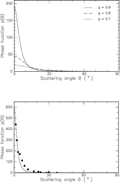
Fig. 2.8. Henyey–Greenstein function for di erent coe cients of anisotropy ranging from g = 0.7 to g = 0.9
Fig. 2.9. Phase function for an 80μm thick sample of aortic wall. The data are fitted to a composite function consisting of an isotropic term u and the anisotropic Henyey–Greenstein function (fit parameters: g = 0.945, u = 0.071). Data according to Yoon et al. (1987)
2.4 Turbid Media |
25 |
where Pi are the Legendre polynomials. In some cases, though, a composite function of an isotropic term u and the Henyey–Greenstein function does fit better to experimental data. According to Yoon et al. (1987), this modified function can be expressed by
|
1 u + (1 −u)(1 −g2) |
(2.29) |
|||||
p(θ) = |
|
|
|
|
|
. |
|
|
(1 + g |
2 |
3/2 |
||||
4π |
|
−2g cosθ) |
|
||||
In Fig. 2.8, the Henyey–Greenstein phase function is graphically shown for di erent values of g. Obviously, it describes the dominant process of scattering in the forward direction very well. In Fig. 2.9, experimental data are plotted for an 80μm sample of aortic tissue. The data are fitted to the modified Henyey–Greenstein function as determined by (2.29) with the parameters g = 0.945 and u = 0.071.
2.4 Turbid Media
In the previous two sections, we have considered the occurrences of either absorption or scattering. In most tissues, though, both of them will be present simultaneously. Such media are called turbid media. Their total attenuation coe cient can be expressed by
αt = α + αs . |
(2.30) |
In turbid media, the mean free optical path of incident photons is thus determined by
Lt = |
1 |
= |
1 |
. |
(2.31) |
|
αt |
|
α + αs |
||||
Only in some cases, either α or αs may be negligible with respect to each other, but it is important to realize the existence of both processes and the fact that usually both are operating. Also, it is very convenient to define an additional parameter, the optical albedo a, by
a = |
αs |
= |
|
αs |
. |
(2.32) |
αt |
|
|||||
|
|
α + αs |
|
|||
For a = 0, attenuation is exclusively due to absorption, whereas in the case of a = 1 only scattering occurs. For a = 1/2, (2.32) can be turned into the equality α = αs, i.e. the coe cients of absorption and scattering are of the same magnitude. In general, both e ects will take place but they will occur in variable ratios.
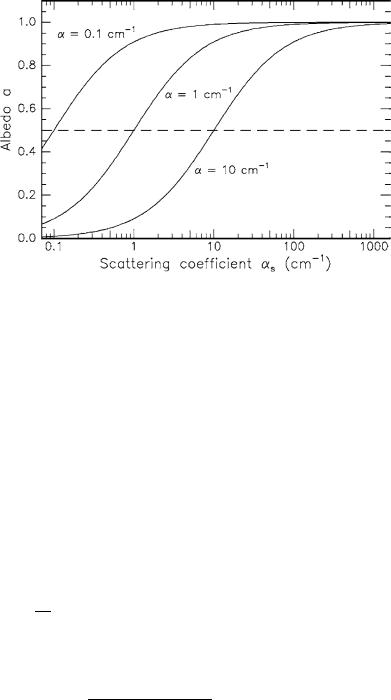
In Fig. 2.10, the albedo is shown as a function of the scattering coe cient. Three di erent absorption coe cients are assumed which are typical for biological tissue. In addition, the value a = 1/2 is indicated. For αs >> α, the albedo asymptotically approaches unity.
26 2. Light and Matter
Fig. 2.10. Optical albedo as a function of scattering coe cient (absorption coe - cient: as labeled). The albedo a = 1/2 is indicated
When dealing with turbid media, another useful parameter is the optical depth d which is defined by
s
d = αt ds , (2.33)
0
where ds denotes a segment of the optical path, and s is the total length of the optical path. In the case of homogeneous attenuation, i.e. a constant attenuation coe cient αt, (2.33) turns into
d = αt s .
The advantage of using albedo a and optical depth d – instead of absorption coe cient α and scattering coe cient αs – is that the former are dimensionless parameters. The information contained in the pair a and d, though, is the same as in the pair α and αs.
When considering turbid media, the normalization of the phase function as given by (2.26) must be altered to
1
4π
p(θ) dω = a ,
4π
since the probability function should approach zero at negligible scattering. Hence, (2.27) and (2.28) are no longer valid and must be replaced by
1 −g2
p(θ) = a (1 + g2 −2g cosθ)3/2 ,

2.5 Photon Transport Theory |
27 |
and
∞
p(θ) = a (2i + 1)gi Pi(cosθ) .
i=0
In the literature, reduced scattering and attenuation coe cients are often dealt with and are given by
αs = αs (1 −g) , |
(2.34) |
and |
|
αt = α + αs , |
(2.35) |
since forward scattering alone, i.e. g = 1, would not lead to an attenuation of intensity. These definitions will turn out to be very useful, especially when discussing the di usion approximation in the next section.
2.5 Photon Transport Theory
A mathematical description of the absorption and scattering characteristics of light can be performed in two di erent ways: analytical theory or transport theory. The first is based on the physics of Maxwell’s equations and is, at least in principle, the most fundamental approach. However, its applicability is limited due to the complexities involved when deriving exact analytical solutions. Transport theory, on the other hand, directly addresses the transport of photons through absorbing and scattering media without taking Maxwell’s equations into account. It is of a heuristic character and lacks the strictness of analytical theories. Nevertheless, transport theory has been used extensively when dealing with laser–tissue interactions, and experimental evidence is given that its predictions are satisfactory in many cases. Therefore, this section is confined to the transport theory of light.
In our presentation, we will follow the excellent review of transport theory given by Ishimaru (1989). The fundamental quantity in transport theory is called the radiance3 J(r,s) and is expressed in units of Wcm−2 sr−1. It denotes the power flux density in a specific direction s within a unit solid angle dω. The governing di erential equation for radiance is called the radiative transport equation and is given by
dJ(drs,s) = −αtJ(r,s) + 4πs |
|
p(s,s )J(r,s ) dω , |
(2.36) |
||
|
|
α |
|
|
|
|
|
|
4π |
|
|
3Note that our definition of radiance di ers from intensity by the extra unit sr−1. We are thus using two di erent symbols J and I, respectively. This mathematically inconvenient distinction becomes necessary, since scattered photons may proceed into any solid angle.