Laser-Tissue Interactions Fundamentals and Applications - Markolf H. Niemz

used to calculate the shock wave pressure p1 as a function of shock speed us. By this means, shock wave pressures – which are usually very di cult to determine – can be derived from measured shock speeds.

Such calculations were performed by Vogel et al. (1994a) for shock waves induced by picosecond and nanosecond pulses. Their results are summarized in Fig. 3.64 where the shock wave pressure is shown in various distances from the center of emission. The initial pressure at the boundary of the laser plasma was 17kbar for 50μJ pulses with a duration of 30ps, whereas it was 21kbar for 1mJ pulses with a duration of 6ns. Although these values are quite similar, the pressure decay is significantly steeper for those shock waves which were induced by the picosecond pulses. In a distance of approximately 50μm from the center of the shock wave emission, their pressure has already dropped to 1kbar, whereas this takes a distance of roughly 200μm when applying nanosecond pulses.

Moreover, it was observed by Vogel et al. (1994a) that the width of shock waves is smaller in the case of the picosecond pulses. They evaluated approximate widths of 3μm and 10μm for shock waves induced by either 30ps or 6ns pulses, respectively. Thus, the energies contained in these shock waves

with shock wave pressure p1, shock wave surface area As, and shock wave width Δr. Due to di erent plasma lengths as shown in Fig. 3.60, we obtain initial values of As 100μm2 for 30ps pulses and As 2500μm2 for 6ns pulses when assuming a focal spot diameter of 4μm. From (3.70), we then find that Es 0.5μJ for 30ps pulses and Es 50μJ for 6ns pulses. Thus, only 1– 5% of the incident pulse energy is converted to shock wave energy, and shock waves from picosecond pulses are significantly weaker than those induced by nanosecond pulses with comparable peak pressures. From the corresponding particle speeds, Vogel et al. (1994a) have calculated a tissue displacement of approximately 1.2μm for 30ps pulses and a displacement of roughly 4μm for 6ns pulses. These rather small displacements can cause mechanical damage on a subcellular level only, but they might induce functional changes within cells.

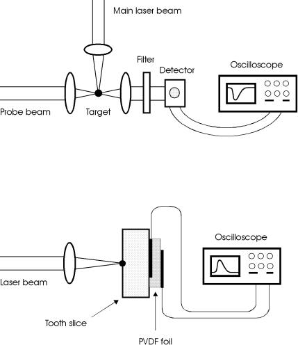
Primarily, there exist two types of experiments which are performed to investigate the dynamics of shock wave phenomena: optical and mechanical measurements. During optical measurements, the shock wave is detected with a weaker probe beam after being generated by the main laser beam. In some setups, an external helium–neon laser or dye laser is used as a probe beam. In other cases, the probe beam is extracted from the main beam by means of a beamsplitter and directed through an optical delay. A decrease in probe beam intensity is detected with a fast photodiode as long as the shock wave passes through the focus of the probe beam. By moving the focus of the probe beam with respect to the site of plasma generation, the propagation of the

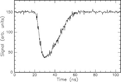
In Figs. 3.67 and 3.68, typical results are shown concerning the detection of acoustic transients. In Fig. 3.67, a shock wave was generated when inducing a plasma inside water by a 30ps pulse from a Nd:YLF laser. A helium–neon laser served as a probe beam being focused at the depth of interest and detected with a fast photodiode. The probe beam is deflected as the shock wave passes through the focus of the probe beam, resulting in a decrease in detected intensity. A steep shock front is seen lasting for approximately 10ns. After another 30ns, the shock wave has completely passed. During its overall duration of roughly 40ns, the shock wave can hardly cause any gross tissue displacement. Thus, further evidence is given that shock wave damage is limited to a subcellular level.

Fig. 3.67. Signal from a helium–neon laser serving as a detector for a shock wave generated in water by a Nd:YLF laser (pulse duration: 30ps, pulse energy: 1mJ)

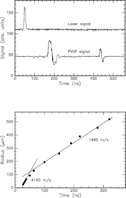
In Fig. 3.68, on the other hand, the voltage signal from a PVDF transducer is shown. In this case, a plasma was induced at the surface of a tooth slice with a thickness of 0.5mm. The detected PVDF signal arrives approximately 130ns after the incident laser pulse, thus corresponding to a velocity of about 3800m/s which is the speed of sound in teeth. The acoustic transient is reflected at the opposite surface of the tooth slice and is again detected after about 2×130ns = 260ns. Taking the round trip through the tooth slice into account, this time delay is related to the same speed of sound.

Since the shock wave loses energy when propagating through a medium, it eventually slows down until it finally moves at the speed of sound. With probe beam experiments as discussed above, traces of the shock wave at di erent

distances from its origin can be measured by moving the focus of the probe beam away from the plasma site. Typical results for such an experiment are shown in Fig. 3.69. From these data, a shock speed of approximately 4160m/s is calculated for the first 30ns. According to Fig. 3.63, this value corresponds to a shock wave pressure of approximately 60kbar. The shock wave then slows down to about 1480m/s – the speed of sound in water – after another 30ns. Therefore, the spatial extent of shock waves is limited to approximately 0.2mm. Similar results were reported by Puliafito and Steinert (1984) and Teng et al. (1987).

3.5.3 Cavitation

Historically, interest in the dynamics of cavitation bubbles started to rise after realizing their destructive e ect on solid surfaces such as ship propellers and other hydraulic equipment. Laser-induced cavitations occur if plasmas are generated inside soft tissues or fluids. By means of the high plasma temperature, the focal volume is vaporized. Thereby, work is done against the outer pressure of the surrounding medium, and kinetic energy is converted to potential energy being stored in the expanded cavitation bubble. Within less than a millisecond, the bubble implodes again as a result of the outer static pressure, whereby the bubble content – typically water vapor and carbon oxides – is strongly compressed. Thus, pressure and temperature rise again to values similar to those achieved during optical breakdown, leading to a rebound of the bubble. Consequently, a second transient is emitted, and the whole sequence may repeat a few times, until all energy is dissipated and all gases are solved by surrounding fluids.

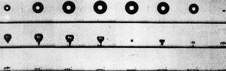
Cavitation bubbles have long been studied by a variety of techniques. The high-speed photographic technique was pioneered by Lauterborn (1972). It is very helpful in visualizing the temporal behavior of the cavitation bubble. High-speed photography is performed at framing rates with up to one million frames per second. A typical sequence of growth and collapse of a cavitation bubble is shown in Fig. 3.70. The bubble appears dark in front of a bright background, because it is illuminated from behind and the light was deflected by its wall. Through the center of the bubble, the illuminating light is transmitted without deflection. In the case shown, a Q-switched ruby laser with pulse energies ranging from 100mJ to 400mJ was used to induce the cavitation bubble. Its maximum diameter reaches a value of 2.05mm at a time delay of approximately 300μs. The end of the first and second collapse is seen in the eighth and thirteenth frames, respectively.

A theory of the collapse of spherical cavitation bubbles was first given by Rayleigh (1917). He derived the relationship

tc

rmax = , (3.71)

0.915 /(pstat −pvap)

144 3. Interaction Mechanisms

Fig. 3.70. Dynamics of cavitation bubble captured with high-speed photography. Pictures taken at 20000 frames per second (frame size: 7.3mm×5.6mm). Reproduced from Vogel et al. (1989) by permission. c 1989 Cambridge University Press

where rmax is the maximum radius of cavitation, tc is the duration of the collapse, is the density of the fluid, pstat is the static pressure, and pvap is the vapor pressure of the fluid. Thus, the time needed for each collapse is proportional to its maximum radius. The latter, on the other hand, is directly related to the bubble energy Eb by means of

according to Rayleigh (1917). This equation states that the bubble energy is given by the product of its maximum volume and the corresponding pressure gradient. The bubble energy is thus readily determined when all kinetic energy has turned into potential energy.

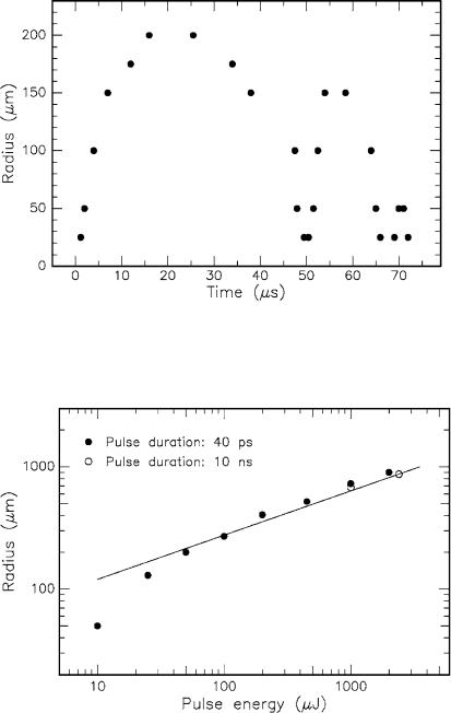
The temporal oscillation of the cavitation bubble can be captured in probe beam experiments as shown in Fig. 3.71. Three complete oscillations are seen. The period of subsequent oscillations decreases in the same manner as their amplitude as already postulated by (3.71). In order to evaluate the dependence of the radius of cavitation on incident pulse energy, probe beam experiments have been performed similar to those discussed for shock wave detection. In Fig. 3.72, some data for picosecond and nanosecond pulses were collected by Zysset et al. (1989). Except for the lowest energy value, their measurements fit well to a straight line with a slope of 1/3. Because of the double-logarithmic scale of the plot, the relation given above by (3.72) is thus experimentally confirmed.

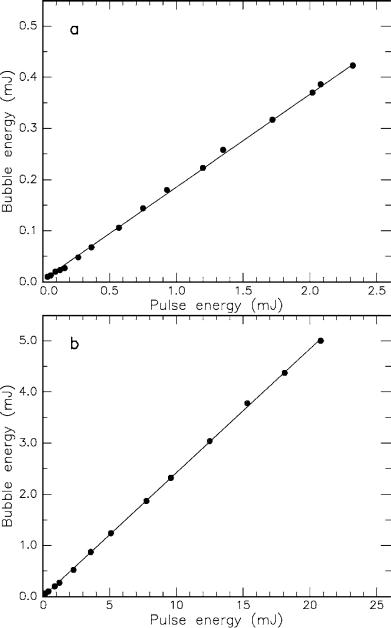
The conversion of incident energy to cavitation bubble energy is summarized in Figs. 3.73a–b. From the slopes, a conversion factor of approximately 19% is obtained for picosecond pulses, whereas it is roughly 24% when applying nanosecond pulses. Moreover, it was observed by Vogel et al. (1989) that the average energy loss of the cavitation bubbles during their first cycle is approximately 84%. The major part of this loss is attributed to the emission of sound. These results were confirmed in theoretical work performed by Ebeling (1978) and Fujikawa and Akamatsu (1980). From (3.72), it can

also be concluded that bubble-induced damage – i.e. the linear extent of the damage zone – scales with the cube root of the contained energy. This is of importance when determining the primary cause of tissue damage. It was observed by Vogel et al. (1990) that tissue damage also scales with the cube root of pulse energy. Thus, cavitations are more likely to induce√damage than shock waves, since shock wave damage should be related to E as can be derived from (3.70) when inserting As r2.

It has been emphasized above that damage of tissue due to shock waves is limited to a subcellular level due to their short displacement lengths of approximately 1–4μm. Since the diameter of cavitation bubbles may reach up to a few millimeters, macroscopic photodisruptive e ects inside tissues are believed to primarily originate from the combined action of cavitation and jet formation which will be discussed next.

3.5.4 Jet Formation

As recently stated by Tomita and Shima (1986), the impingement of a highspeed liquid jet developing during the collapse of a cavitation bubble may lead to severe damage and erosion of solids. Jet formation was first investigated and described by Lauterborn (1974) and Lauterborn and Bolle (1975) when producing single cavitation bubbles by focusing Q-switched laser pulses into fluids. When cavitation bubbles collapse in the vicinity of a solid boundary, a high-speed liquid jet directed toward the wall is produced. If the bubble is in direct contact with the solid boundary during its collapse, the jet can cause high-impact pressure against the wall. Thus, bubbles attached to solids have the largest damage potential.

Jet formation has been thoroughly studied by means of high-speed photography as introduced above. The temporal behavior of cavitation and jet formation is shown in Fig. 3.74. A cavitation bubble was generated near a solid boundary – a brass block located at the bottom of each frame and visible by a dark stripe – and captured with high-speed photography. Jet formation toward the brass block is observed during the collapse of the bubble. Jet velocities of up to 156m/s were reported by Vogel et al. (1989). The water hammer pressure corresponding to such a velocity is approximately 2kbar. If the distance between the cavitation bubble and solid boundary is further decreased as seen in the bottom sequence of Fig. 3.74, a counterjet is formed which points away from the solid boundary.

What is the origin of jet formation, and why does it only occur near a solid boundary? To answer these questions, let us take a closer look at the collapse of a cavitation bubble. When the bubble collapses due to external pressure, the surrounding fluid is accelerated toward the center of the bubble. However, at the side pointing to the boundary there is less fluid available. Hence, the collapse takes place more slowly at this side of the bubble. This e ect ultimately leads to an asymmetric collapse. At the faster collapsing side, fluid particles gain additional kinetic energy, since the decelerating force – i.e. the