Micro-Nano Technology for Genomics and Proteomics BioMEMs - Ozkan

universal primer can capture the unique sequences of the inserts. Fluorescent dyes used to detect the order of nucleotides (bases) are attached either to the universal primer (“dye primer sequencing”) or to the dideoxynucleoside triphosphates (“dye terminator sequencing”). In the sequencing reactions, a mixture of molecular copies of the DNA template is generated in which subsets of the mixture have terminated at each nucleotide position in the original template. Once a ddNTP is used as a building block instead of a dNTP the polymerase cannot incorporate additional bases onto that molecular chain of DNA (hence “termination”). As a result of the random incorporation of ddNTPs, the completed sequencing reaction mixture contains a nested set of molecules with lengths corresponding to the distance between the universal primer and each base position in the insert sequence. After 1990, sequencing reactions were usually performed in automated thermocycler machines in a 96-well format.

Detection: Using electrophoresis to separate the mixture of molecules based on their size, and lasers to detect the incorporated fluorescent dye as the molecules of a given size pass by the detector. Gel electrophoresis, used in the early days of the project (1990–1998), was supplanted by capillary electrophoresis in the later stages (1998–2003). Electrophoresis and detection were performed with automated fluorescent DNA sequencers. The most commonly used commercial machines were the Applied Biosystems 373A (1990–1996), 377 (1995–1999), 3700 (1998–2002) and 3730 (2002-present), and the Molecular Dynamics/Amersham MegaBACE 1000 and 4000 capillary sequencers (1998–present).

Base-calling: Using software to translate the dye peaks in gel or capillary images into the corresponding bases, relying upon signal-to-noise ratios and peak spacing to make the proper call. When gel electrophoresis was used, adjacent lanes of dye peaks had to be properly delineated prior to running the base-calling program. Because of crossover mistakes, the automated lane-tracking output usually needed to be tweaked by a technician using a manual override function of the software. Retracking a 96-lane gel image could take up to an hour.

Data curation: Copying files of base-called reads to a suitable project directory pertaining to the source clone being sequenced.

Typically, genome centers used automated procedures with varying degrees of sophistication for subclone DNA template preparation, sequencing reaction set-up, sequencing, detection, and base-calling. However, the initial steps of source clone DNA preparation and shotgun library construction (fragmentation, size selection, and subcloning) were hands-on, fussy, and frequently caused difficulties due to irreproducible or non-robust protocols. The following intermittent problems were the bane of a shotgun library construction manager’s existence:

Non-random fragmentation of the source clone;

Low yield in the ligation/transformation step;

Large amounts of contaminating E. coli sequence;

A recombinant “clone from hell” contaminating a ligation or transformation reagent such that a high percentage of the clones in the shotgun library would have the same sequence;

Average Daily Quality

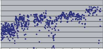
FIGURE 11.5. Fluctuations in data quality. Each dot represents an average of Phred quality scores for all reads on all machines at the Multimegabase Sequencing Center (courtesy of Scott Bloom). Quality improved with a change in sequencing reaction precipitation procedure (June, 2001), and a switch from the ABI 3700 to the 3730 sequencer (September, 2003).

Libraries made from a “wrong” clone due to erroneous mapping information or a mistake in source clone retrieval from the clone library or a deletion of part of the insert DNA during growth of the source clone.

To detect these potential problems, a small test set of 96 reads would usually be obtained before committing to sequence a given shotgun library at high redundancy. The test set of sequence reads was also useful for verifying the map position of the source clone and for staking a claim to a chromosomal region, as will be discussed below.

Although the sequencing and detection steps were straightforward and amenable to high-throughput, multiple things could go wrong such as impure DNA templates, reagents going “bad”, low or noisy signal in the detection of the fluorescent dyes, streaky gels, blank lanes, machine breakdown, sample-tracking errors, computer disk failure and the like. Thus, consistently generating high quality sequence data was difficult due to the plethora of variables in the system (Figure 11.5).

Moreover, managing the data, equipment and personnel was a perpetual juggling act. Centers were constantly recruiting and training technicians because employees would tire of boring, repetitive work and quit or transfer to a different part of the project. Some problems simply could not be anticipated or controlled. When Rick Wilson, the highly successful director of sequencing at the Washington University of St Louis genome center was queried as to his biggest challenge for data generation, he immediately responded with “romances in the lab.” At Whitehead, one of the biggest problems was alleged to be handling the trash. At the Multimegabase Sequencing Center, the laboratory changed institutions twice (Caltech to University of Washington to Institute for Systems Biology) and moved five times over the course of 10 years.

11.2.2.3. Assembly In shotgun sequencing, a “consensus” sequence is constructed from the sequences of overlapping reads derived from randomly generated fragments of the

subclone 17G1

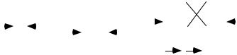
FIGURE 11.6. Plasmid end pairs. Paired ends of sublone 14H9 indicate that contig 47 is adjacent to contig 13. In subclone 2C4, the paired ends are too far apart, and in subclone 17G1, the paired ends are in the same orientation, both of which problems indicate a misassembly in contig 47.

scores determined the best matches among them. After assembly, each base was given a “Phrap score,” reflecting the extent to which the base was confirmed by bases in other reads (e.g., confirmation from the opposite strand was given more weight than confirmation from the same strand.) Rather than determining a consensus based on majority rule, a “consensus” sequence for the source clone was determined by choosing the base with the highest Phred/Phrap score for each position. As a result, the Phrap assembler generated longer contigs with more accurate consensus sequences because it used the quality scores to select the best data.

Both before and since Phrap, there have been numerous sequence assemblers built for the purpose of aligning shotgun reads and constructing contigs (e.g., [1, 4, 5, 20, 29, 31, 48]). Using their assembly engine of choice, the software typically performed the following steps:

Read processing: Assign quality scores to bases or trim reads.

Assembly: Perform pairwise alignments between reads.

Construct contigs: Represent the overlapping reads as a consensus sequence supported by an array of reads, with the starting and ending position of each read oriented relative to the consensus sequence.

In addition to these steps, some assemblers were able to order and orient contigs based on information derived from paired clone end sequences. That is, if both ends (i.e., vectorinsert joints) of a 1–4 kb plasmid insert were sequenced, then the beginnings of those paired reads needed to be 1–4 kb apart in the assembled sequence with the sequences pointing towards each other (Figure 11.6). Using a contig editor, that is, an editor designed to display the results of the assembly, the order and orientation of contigs based on paired ends could also be determined manually.

Assuming highly redundant read coverage, the major pitfall of assembly was misassembled reads due to repetitive content in the insert of the source clone. If the sequence similarity between repeats averaged 98% or less over a kb, Phrap could generally produce the correct answer. With lower coverage or repeats of higher sequence similarity, reads from the repeats would “pile up” in a misassembled contig and have to be sorted out in the finishing phase.

11.2.2.4. Finishing The sequence of a source clone was considered finished if a contiguous consensus sequence was accurate at each base position and the underlying

assembly was correct. The accepted standard of accuracy was 99.99%, or 1 error on average in 10,000 bases. In order for a finished clone to be part of a chromosomal tiling path, further validation was required as to the integrity of the source clone DNA (i.e., no deletions or rearrangements) and the proper chromosomal assignment based on FISH, genetic marker content, or convincing overlaps with other validated clones.

Turning a set of assembled contigs into a finished sequence typically involved successive iterations of the following steps until a contiguous and accurate consensus sequence was obtained:

Additional sequencing: Filling gaps and improving poor quality portions of the consensus due to noisy read data or sparse coverage in the assembly required the gathering of additional sequence data either by obtaining more shotgun reads, or resequencing selected clones using a different chemistry, or extending the length of a read with a custom oligonucleotide primer, or using the polymerase chain reaction (PCR) to generate sequence-ready DNA from a plasmid subclone, the source clone itself, or even human genomic DNA.

Reassembly: Incorporating additional sequence data into a set of already assembled reads or repeating the entire assembly de novo upon the addition of new sequence reads.

Editing: Determining the order and orientation of contigs, performing base-calling judgments in regions of ambiguity, breaking apart misassembled contigs, and joining overlapping contigs. This was typically done by an experienced “finisher” using a sequence contig display editor with features allowing for base-call overrides, complementation of contigs, removal of selected reads from contigs, the capacity to split contigs apart, and the creation of “fake” reads to glue contigs together.

Once the sequence of a source clone was provisionally finished, it needed to be validated to ensure that the assembly was correct. Validation procedures included satisfaction of the distance constraints imposed by paired end sequences (Figure 11.6), agreement with sequences of overlapping clones, and comparison of restriction digest fingerprint patterns predicted by the sequence to the experimentally determined patterns of the source clone.

Like mapping, finishing was a slow and laborious process requiring skilled personnel. To speed it up, several centers instituted variants of a strategy called “autofinish” [17]. Using a specified set of rules (for example, “Additional sequence data must be generated for any region in the consensus supported by two or fewer reads.”) the autofinish software was designed to create a list of reads and suggested strategies to be used for generating additional sequence data. Skilled finishers stepped in after the assembly project had been subjected to several rounds of autofinish. While the finishing of most source clone sequences was straightforward, some clones posed problems, most typically gaps for which no sequence could be obtained using a variety of strategies, or misassemblies due to sequence repeats resulting from gene duplications or low complexity DNA3. Difficult clones often took months and sometimes years to finish!

In the last two years of the genome project, finishing was a serious problem due to a backlog of assembled source clones and political pressure to get the genome done by the deadline of April 2003. In addition to autofinish, genome centers dealt with the problem by

3Examples of low complexity DNA are homopolymer runs or long stretches of a short repeating unit of DNA, e.g., three kilobases of a consecutive 40 base repeat with minor variations.

Genome Sequence Data Base, now extinct) in the US, EMBL (European Molecular Biology Laboratory) in Europe or DDBJ (DNA Database of Japan). Data submitted to any one of these databases were also displayed by the others. When the genome project began to scale up, the International Consortium committed itself to releasing sequences prior to finishing, in a form called “working draft” [9]. A new division of the databases, called HTGS (high throughput genome sequence) was established into which assembled contigs from a source clone were to be deposited within a day of their generation. To indicate the extent of completion, annotation tags for three “phases” were defined:

Phase 1 indicates a set of unordered assembled contigs;

Phase 2 indicates a set of ordered and oriented contigs;

Phase 3 indicates a finished sequence.

Annotation tags were also included for the source clone and library ID, the submitting genome center, and the chromosomal location of the sequence. Even though the assembly and/or the chromosomal map position of the working draft sequences were wrong in some instances, the genome community’s decision to release the sequence data prior to finishing provided enormous benefit to researchers searching for disease genes.

With the increased use of the World Wide Web in the mid-90s, data became increasingly accessible to anyone interested. In addition to the central public databases, genome centers typically established their own web sites for sharing data and protocols. Over time, the National Center for Biotechnology Information (NCBI) and the University of California, Santa Cruz in the US, the European Bioinformatics Institute (EBI) in Great Britain, and several other organizations and companies have gathered and integrated a rich assortment of resources to facilitate understanding and utilization of the genome sequence data4. Along with the sequences themselves, these web sites include maps, gene identifications, gene expression results, cross-species comparisons, gene function annotations, and the like.

11.3. CHALLENGES FOR SYSTEMS INTEGRATION

At the inception of the human genome project in the late ‘80s, there was significant controversy over whether sequencing the genome was worth doing and if it could actually be done. At the time, the longest contiguous stretch of DNA that had been sequenced was well under 100 kb [6]. Automated fluorescent DNA sequencing had recently been invented and commercialized, representing a vast improvement over radioactive sequencing. Nonetheless, sequencing 3 billion bases would more than challenge the then-current methodologies and would likely incur significant cost. But with great optimism, it was assumed that cheap and effective new strategies for sequencing would emerge as they were needed. In the original design of the genome project, projected to last from 1990–2005, physical maps of the chromosomes would be constructed during the first 5–10 years. In parallel with this effort, revolutionary sequencing strategies leading to orders of magnitude increases in throughput

4See http://www.ncbi.nlm.nih.gov/ for NCBI; http://genome.ucsc.edu for University of California Santa Cruz; and http://www.ebi.ac.uk/ for EBI.

would be invented and implemented5. With the maps and the methods in place, the genome would then be sequenced during the last 5 years in high-throughput factory-style operations.

This is not exactly how things turned out. Sequence-ready physical maps were not constructed at the outset and revolutionary methods for sequencing did not appear. Nonetheless, the genome was sequenced two years ahead of schedule1. Along the way, the sequencing centers faced numerous challenges for systems integration due to the pioneering nature, complexity, and scale of the human genome project. These challenges fall into two broad categories: developing and applying the methodologies for sequencing source clones, and achieving overall project coordination for finishing a master sequence for each chromosome.

Between 1990 and 1996, significant progress was made regarding the choice of an overall strategy and refinement of specific sets of procedures for sequencing individual source clones. Once a mature set of procedures for shotgun sequencing was developed, the scale-up of the genome project could begin in 1997 and accelerate rapidly in 1999. While numerous challenges attended the day-to-day implementation of sequencing methods as well as the knotty issues of managing and tracking the data, from a historical perspective, the more interesting debates pertained to the initial acceptance and refinement of shotgun sequencing procedures.

Project coordination challenges came into play most noteworthily after year 2000 when the focus shifted to figuring out how to get the entire human genome sequenced, assembled, and validated. Turning multitudinous source clone sequences into polished chromosome sequences required the development of centralized resources and significant cooperation among the several genome centers doing the finishing. These challenges will be discussed in a subsequent section.

11.3.1. Methodological Challenges for Sequencing Source Clones: 1990–1997

Returning to the pipeline analogy, each of the genome centers needed to design an approach to sequencing that was capable of processing large numbers of samples through successive series of steps. The best approaches would possess the following virtues:

Scalability: Procedures that worked on a small scale needed to carry over to a large scale if they were to be useful. Reducing the number of steps, automating as many steps as possible, increasing the sample-processing capacity for each step, instituting fail-safe sample-tracking procedures, and improving the robustness of each step all conduced to more scalable procedures.

Cost-effectiveness: Cost-effective procedures were those with high success rates using minimal amounts of expensive reagents, equipment, labor and time.

Good data quality: Because several steps were required to get from a mapped source clone to finished sequence, producing high quality data at each step increased the efficiency of the overall process due to greater yields and less need for backtracking.

Elimination of bottlenecks: No matter how speedy or high-throughput any individual step was be made to be, the rate of production of the overall process could be no faster

5For the text of the various 5 year plans for the human genome project, see: http://www.ornl.gov/sci/techresources/ Human Genome/hg5yp/index.shtml

than the slowest steps. Long “cycle times” for sequencing source clones increased the managerial complexity of the overall operation.

Adaptability: Changing technologies and policies mandated that the sequencing pipeline be somewhat flexible.

In an ideal world, optimization of all these virtues would converge on the same set of procedures, and that happened with shotgun sequencing. Along the way to developing a mature strategy, though, there were various disagreements and failed approaches, some of which will be presented herein.

11.3.1.1. Why Revolutionary Sequencing Technologies Never Got off the Ground

During the early ‘90s, several novel strategies for sequencing were proposed and attempted for the purpose of replacing electrophoresis-based automated fluorescent sequencing methods of detection with higher throughput approaches. At the time, the Applied Biosystems 373A sequencer produced reads of about 450 good bases in 14–16 hour runs on gels loaded with 36 or 48 lanes of sequencing reactions. At 15 reads/kb, one needed either many expensive sequencers or many days to produce enough sequence reads to assemble a 40 kb cosmid with this level of throughput. Sequencing by hybridization [13], sequencing by mass spectrometry [32], and multiplex Maxam-Gilbert sequencing [7] were among the strategies tried. These methods and others suffered from one or more of the following problems: overly high error rates; short read lengths; inability to automate sample processing; only model templates worked; or no easy way to do base-calling. Most of the revolutionary methods were not capable of producing even a tiny amount of human genome sequence data, let alone able to scale.

Electrophoresis-based detection technologies, in the meantime, improved incrementally. The number of lanes loaded onto a sequencer went from 24 to 36 to 48 to 72 to 96. The Applied Biosystems 377 sequencer introduced in the mid-90s reduced the gel run time to 7–9 hours, thus allowing for 2–3 runs a day. Improvements in the polymerases [46] and dyes [41] produced longer reads of higher quality. By 1997, one ABI 377 produced 192 reads averaging about 650 bases (124,800 bases) in a day, about an 8-fold improvement over 1992 technology (16,200 bases). In 1998, capillary electrophoresis (ABI 3700, MagaBace 1000) reduced the machine run time to a couple of hours and obviated the need for manual lane-tracking prior to base-calling. By 2003, the Applied Biosystems 3730 capillary sequencer produced about 450,000 bases a day, close to a 30-fold improvement over 1992 technology. Even though the changes were incremental as they occurred, the overall effect of improved procedures for automated fluorescent sequencing were dramatic in terms of throughput, data quality, and cost-savings.

As important as cranking out bases of high quality sequence, use of the automated sequencers integrated well with the use of robotic approaches to the upstream steps of the sequencing pipeline. By the mid-90s, the incentive to supplant electrophoresis-based detection technology with revolutionary alternative approaches was lost, and it made increasing sense to get on with the sequencing of the genome using a technology that worked [35]. Thus, the scale-up began in 1997, four years ahead of schedule. (Interestingly, in recent years there has been a resurgent interest in developing new sequencing technologies primarily aimed at resequencing portions of the genome for detecting sequence variations. A discussion of these is beyond the scope of this review.)

sequencing,” said geneticist Maynard Olson to the author of this review circa 1993, “is like buying 8 copies of a prefabricated house and constructing one house from the parts— it’s inelegant and inefficient.” Especially in light of the seemingly low-throughput of the sequencers and the significant expense of the reagents, having to generate subclones and sequencing reads sufficient to cover a source clone about eight times over seemed like a wasteful approach in the early ‘90s. Although hard to believe in hindsight, the resistance to high-redundancy shotgun sequencing was fairly vociferous in the early days of the genome project. To reduce the redundancy, more directed approaches were proposed. One of these involved using transposons to map plasmid subclone inserts, the idea being that sequencing an array of ordered inserts would require the acquisition of less sequence data (even though an additional mapping step was introduced) [45]. Other strategies advocated extensive use of oligonucleotide-directed sequencing to extend the length of the reads obtainable from phage or plasmid subclones.

Although intuitively appealing, alternatives to high-redundancy shotgun sequencing were gradually abandoned for several reasons. First, shotgun sequencing reduced the burden of finishing by vastly improving the quality of the input data. With shotgun sequencing there were fewer gaps to fill and more options for resolving discrepancies among reads, thus reducing the additional work required for resequencing. Moreover, assembly errors due to gene duplications and other repeats in the source clone could be detected and often resolved by a rearrangement of the sequencing reads. Second, the steps of shotgun sequencing were more automatable because samples could be processed in a 96-well or 384-well format using robots. Introduction of mapping or directed sequencing steps required handling and tracking individual samples. Third, shotgun sequencing was more tolerant of failure. If 96-well plates of templates or sequencing reactions were dropped on the floor or flipped into the opposite orientation or otherwise lost or mislabeled this had little effect on the downstream steps. These problems, as well as failed sequencing reactions or gel runs, could be overcome by obtaining more random reads from the shotgun library. Most genome centers built a standard failure rate into their calculations of numbers of reads/kb to sequence. In contrast to shotgunning, any procedure that relied on particular individual samples surviving through all of the steps made failures more difficult to deal with and recover from. Fourth, shotgun sequencing was fast. Once a shotgun library was made, the subsequent steps of DNA template preparation, sequencing, and assembly could happen in a few days thanks to process automation. Thus in the end, shotgun sequencing turned out to be more scaleable, cheaper, and easier to do than any of the alternative strategies.

11.3.1.3. How Shotgun Sequencing Involved Trade-Offs Within the basic framework of shotgun sequencing, genome centers had to make tactical decisions based on cost, efficiency, and data quality.

Level of redundancy: Beyond a certain point, additional shotgun reads would fail to improve an assembly and the project would need to go into finishing. Short of that point (about 10-fold effective redundancy with 500 base reads) accumulation of more reads would help for assembly and finishing, but sequence reads were costly in terms of reagents and equipment usage. Therefore, it was tempting to accumulate shotgun reads only up to about 5-fold redundancy. Centers that shortchanged on shotgun reads