most once on a path; but some non-terminal nodes may be labelled with , the exclusive-or operation. The meaning is that the function represented by that node is the exclusive-or of the boolean functions determined by its children. Parity OBDDs have similar algorithms for apply, restrict, etc. with the same performance, but they do not have a canonical form. Checking for equivalence cannot be done in constant time. There is, however, a cubic algorithm for determining equivalence; and there are also e cient probabilistic tests. Another variation of OBDDs allows complementation nodes, with the obvious meaning. Again, the main disadvantage is the lack of canonical form.

One can also allow non-terminal nodes to be unlabelled and to branch to more than two children. This can then be understood either as nondeterministic branching, or as probabilistic branching: throw a pair of dice to determine where to continue the path. Such methods may compute wrong results; one then aims at repeating the test to keep the (probabilistic) error as small as desired. This method of repeating probabilistic tests is called probabilistic amplification. Unfortunately, the satisfiability problem for probabilistic branching OBDDs is NP-complete. On a good note, probabilistic branching OBDDs can verify integer multiplication.

The development of extensions or variations of OBDDS which are customised to certain classes of boolean functions is an important area of ongoing research.

6.3 Symbolic model checking

The use of BDDs in model checking resulted in a significant breakthrough in verification in the early 1990s, because they have allowed systems with much larger state spaces to be verified. In this section, we describe in detail how the model-checking algorithm presented in Chapter 3 can be implemented using OBDDs as the basic data structure.

The pseudo-code presented in Figure 3.28 on page 227 takes as input a CTL formula φ and returns the set of states of the given model which satisfy φ. Inspection of the code shows that the algorithm consists of manipulating intermediate sets of states. We show in this section how the model and the intermediate sets of states can be stored as OBDDs; and how the operations required in that pseudo-code can be implemented in terms of the operations on OBDDs which we have seen in this chapter.

We start by showing how sets of states are represented with OBDDs, together with some of the operations required. Then, we extend that to the representation of the transition system; and finally, we show how the remainder of the required operations is implemented.

Model checking using OBDDs is called symbolic model checking. The term emphasises that individual states are not represented; rather, sets of states are represented symbolically, namely, those which satisfy the formula being checked.

6.3.1 Representing subsets of the set of states

Let S be a finite set (we forget for the moment that it is a set of states). The task is to represent the various subsets of S as OBDDs. Since OBDDs encode boolean functions, we need somehow to code the elements of S as boolean values. The way to do this in general is to assign to each element s S a unique vector of boolean values (v1, v2, . . . , vn), each vi {0, 1}. Then, we represent a subset T by the boolean function fT which maps (v1, v2, . . . , vn) onto 1 if s T and maps it onto 0 otherwise.

There are 2n boolean vectors (v1, v2, . . . , vn) of length n. Therefore, n should be chosen such that 2n−1 < |S| ≤ 2n, where |S| is the number of elements in S. If |S| is not an exact power of 2, there will be some vectors which do not correspond to any element of S; they are just ignored. The function fT : {0, 1}n → {0, 1} which tells us, for each s, represented by (v1, v2, . . . , vn), whether it is in the set T or not, is called the characteristic function of T .

In the case that S is the set of states of a transition system M = (S, →, L) (see Definition 3.4), there is a natural way of choosing the representation of S as boolean vectors. The labelling function L : S → P(Atoms) (where P(Atoms) is the set of subsets of Atoms) gives us the encoding. We assume a fixed ordering on the set Atoms, say x1, x2, . . . , xn, and then represent s S by the vector (v1, v2, . . . , vn), where, for each i, vi equals 1 if xi L(s) and vi is 0 otherwise. In order to guarantee that each s has a unique representation as a boolean vector, we require that, for all s1, s2 S, L(s1) = L(s2) implies s1 = s2. If this is not the case, perhaps because 2|Atoms| < |S|, we can add extra atomic propositions in order to make enough distinctions (Cf. introduction of the turn variable for mutual exclusion in Section 3.3.4.)

From now on, we refer to a state s S by its representing boolean vector (v1, v2, . . . , vn), where vi is 1 if xi L(s) and 0 otherwise. As an OBDD, this state is represented by the OBDD of the boolean function l1 · l2 · · · · · ln, where li is xi if xi L(s) and xi otherwise. The set of states {s1, s2, . . . , sm} is represented by the OBDD of the boolean function

(l11 · l12 · · · · · l1n) + (l21 · l22 · · · · · l2n) + · · · + (lm1 · lm2 · · · · · lmn)

where li1 · li2 · · · · · lin represents state si.

s2

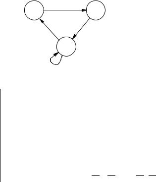
Figure 6.24. A simple CTL model (Example 6.12).

S(1, 0), (0, 1), (0, 0) x1 · x2 + x1 · x2 + x1 · x2

Figure 6.25. Representation of subsets of states of the model of Figure 6.24.

The key point which makes this representation interesting is that the OBDD representing a set of states may be quite small.

Example 6.12 Consider the CTL model in Figure 6.24, given by:

def

S = {s0, s1, s2}

def

→ = {(s0, s1), (s1, s2), (s2, s0), (s2, s2)}

def

L(s0) = {x1}

def

L(s1) = {x2}

def

L(s2) = .

Note that it has the property that, for all states s1 and s2, L(s1) = L(s2) implies s1 = s2, i.e. a state is determined entirely by the atomic formulas true in it. Sets of states may be represented by boolean values and by boolean formulas with the ordering [x1, x2], as shown in Figure 6.25.

Notice that the vector (1, 1) and the corresponding function x1 · x2 are unused. Therefore, we are free to include it in the representation of a subset

Figure 6.26. Two OBDDs for the set {s0, s1} (Example 6.12).

of S or not; so we may choose to include it or not in order to optimise the size of the OBDD. For example, the subset {s0, s1} is better represented by the boolean function x1 + x2, since its OBDD is smaller than that for x1 · x2 + x1 · x2 (Figure 6.26).

In order to justify the claim that the representation of subsets of S as OBDDs will be suitable for the algorithm presented in Section 3.6.1, we need to look at how the operations on subsets which are used in that algorithm can be implemented in terms of the operations we have defined on OBDDs. The operations in that algorithm are:

Intersection, union and complementation of subsets. It is clear that these are represented by the boolean functions ·, + and ¯ respectively. The implementation via OBDDs of · and + uses the apply algorithm (Section 6.2.2).

The functions

pre (X) = {s S | exists s , (s → s and s X)}

(6.4)

pre (X) = {s | for all s , (s → s implies s X)}.

The function pre (instrumental in SATEX and SATEU) takes a subset X of states and returns the set of states which can make a transition into X. The function pre , used in SATAF, takes a set X and returns the set of states which can make a transition only into X. In order to see how these are implemented in terms of OBDDs, we need first to look at how the transition relation itself is represented.

6.3.2 Representing the transition relation

The transition relation → of a model M = (S, →, L) is a subset of S × S. We have already seen that subsets of a given finite set may be represented as OBDDs by considering the characteristic function of a binary encoding.

Just like in the case of subsets of S, the binary encoding is naturally given by the labelling function L. Since → is a subset of S × S, we need two copies of the boolean vectors. Thus, the link s → s is represented by the pair of

Figure 6.27. The truth table for the transition relation of Figure 6.24 (see Example 6.13). The left version shows the ordering of variables

[x1, x2, x1, x2], while the right one orders the variables [x1, x1, x2, x2] (the rows are ordered lexicographically).

boolean vectors ((v1, v2, . . . , vn), (v1, v2, . . . , vn)), where vi is 1 if pi L(s) and 0 otherwise; and similarly, vi is 1 if pi L(s ) and 0 otherwise. As an

OBDD, the link is represented by the OBDD for the boolean function

(l1 · l2 · · · · · ln) · (l1 · l2 · · · · · ln)

and a set of links (for example, the entire relation →) is the OBDD for the + of such formulas.

Example 6.13 To compute the OBDD for the transition relation of Figure 6.24, we first show it as a truth table (Figure 6.27 (left)). Each 1 in the final column corresponds to a link in the transition relation and each 0 corresponds to the absence of a link. The boolean function is obtained by taking the disjunction of the rows having 1 in the last column and is

f → def= x1 · x2 · x1 · x2 + x1 · x2 · x1 · x2 + x1 · x2 · x1 · x2 + x1 · x2 · x1 · x2.

(6.5)

It turns out that it is usually more e cient to interleave unprimed and primed variables in the OBDD variable ordering for →. We therefore use