

72 |
1 Propositional logic |
|
|
“5” = entire formula |
“5” ¬ |
|
“4”= ”3” → ”2” |
“4” ¬ |
|
“3” = p q → r |
|
|
|
|
|
“2” = p → ”1” |
|
|
“1” = q → r |
|
|
|
¬ |
“2”¬
¬
“3”¬
“1”¬
¬
p |
q |
r |
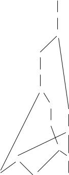
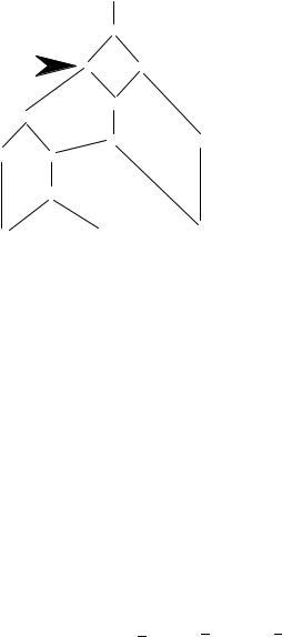
Figure 1.15. The DAG for the translation of ¬((p q → r) → p → q → r). Labels ‘‘1’’ etc indicate which nodes represent what subformulas.
such φ are unsatisfiable. This SAT solver has a linear running time in the size of the DAG for T (φ). Since that size is a linear function of the length of φ – the translation T causes only a linear blow-up – our SAT solver has a linear running time in the length of the formula. This linearity came with a price: our linear solver fails for all formulas of the form ¬(φ1 φ2).
1.6.2 A cubic solver
When we applied our linear SAT solver, we saw two possible outcomes: we either detected contradictory constraints, meaning that no formula represented by the DAG is satisfiable (e.g. Fig. 1.16); or we managed to force consistent constraints on all nodes, in which case all formulas represented by this DAG are satisfiable with those constraints as a witness (e.g. Fig. 1.13). Unfortunately, there is a third possibility: all forced constraints are consistent with each other, but not all nodes are constrained! We already remarked that this occurs for formulas of the form ¬(φ1 φ2).
1.6 SAT solvers |
|
73 |
||
|
|
¬ |
|
1: T |
|
|
¬ |
|
2: F |
|
|
|
|
3: T |
|
4: T ¬ |
|
|
|
|
5: F ¬ |
|
|
|
|
6: T |
|
|
|
its conjunction parent |
7: T ¬ |
¬ |
|
|
and frr force F |
|
|
4: T |
|
its children and |
|
8: F ¬ |
|
|
ti force T |
|
|
|
5: F |
– a contradiction |
|
|
|
|
|
|
9: T |
|
|
|
|
|
¬ |
10: T |
7: T p |
10: T |
q |
r |
11: F |
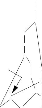
Figure 1.16. The forcing rules, applied to the DAG of Figure 1.15, detect contradictory constraints at the indicated node – implying that the initial constraint ‘1:T’ cannot be realized. Thus, formulas represented by this DAG are not satisfiable.
Recall that checking validity of formulas in CNF is very easy. We already hinted at the fact that checking satisfiability of formulas in CNF is hard. To illustrate, consider the formula
((p (q r)) ((p ¬q) ((q ¬r) ((r ¬p) (¬p (¬q ¬r))))))
(1.11)
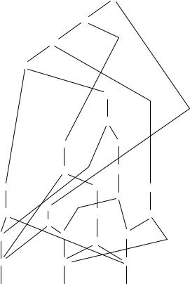
in CNF – based on Example 4.2, page 77, in [Pap94]. Intuitively, this formula should not be satisfiable. The first and last clause in (1.11) ‘say’ that at least one of p, q, and r are false and true (respectively). The remaining three clauses, in their conjunction, ‘say’ that p, q, and r all have the same truth value. This cannot be satisfiable, and a good SAT solver should discover this without any user intervention. Unfortunately, our linear SAT solver can neither detect inconsistent constraints nor compute constraints for all nodes. Figure 1.17 depicts the DAG for T (φ), where φ is as in (1.11); and reveals
74 |
1 Propositional logic |
2: T
3: T
4: T
|
|
3: T ¬ |
|
|
4: F |
5: T |
¬ |
|
|
|
2: T |
6: F |
|
¬ |
|
|
3: F |
|
¬ |
¬ |
|
¬ |
¬ |
|
p |
q |
1: T
5:T ¬
6:F
¬
¬
¬
¬
4: T ¬
5: F
¬
¬
r
Figure 1.17. The DAG for the translation of the formula in (1.11). It has a -spine of length 4 as it is a conjunction of five clauses. Its linear analysis gets stuck: all forced constraints are consistent with each other but several nodes, including all atoms, are unconstrained.
that our SAT solver got stuck: no inconsistent constraints were found and not all nodes obtained constraints; in particular, no atom received a mark! So how can we improve this analysis? Well, we can mimic the role of LEM to improve the precision of our SAT solver. For the DAG with marks as in Figure 1.17, pick any node n that is not yet marked. Then test node n by making two independent computations:
1.determine which temporary marks are forced by adding to the marks in Figure 1.17 the T mark only to n; and
2.determine which temporary marks are forced by adding, again to the marks in Figure 1.17, the F mark only to n.
1.6 SAT solvers |
75 |
1: T
|
|
2: T |
|
|
|
|
3: T |
|
|
|
|
|
4: T |
|
|
|
|
|
|
|
5: T ¬ |
|
|
|
|
|
6: F |
|
|
|
|
3: T ¬ |
|
b:F ¬ |
|
temporary T mark |
|
|
|
|
|
at test node; |
4: F |
|
c:T ¬ |
|
|
explore consequences |
|
|
|||
5: T |
¬ |
2: T |
i:F ¬ |
d:F |
4: T ¬ |
6: F |
|
¬ |
h:T ¬ |
|
5: F |
|
3: F |
|
c:T ¬ |
||
a:T |
¬ |
e:F ¬ |
g:F |
||
b:F |
¬ |
f:T ¬ |
|
b:F |
¬ |
c:T |
p |
g:F q |
|
c:T |
r |
contradictory constraints
at conjunction
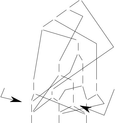
Figure 1.18. Marking an unmarked node with T and exploring what new constraints would follow from this. The analysis shows that this test marking causes contradictory constraints. We use lowercase letters ‘a:’ etc to denote temporary marks.
If both runs find contradictory constraints, the algorithm stops and reports that T (φ) is unsatisfiable. Otherwise, all nodes that received the same mark in both of these runs receive that very mark as a permanent one; that is, we update the mark state of Figure 1.17 with all such shared marks.
We test any further unmarked nodes in the same manner until we either find contradictory permanent marks, a complete witness to satisfiability (all nodes have consistent marks), or we have tested all currently unmarked nodes in this manner without detecting any shared marks. Only in the latter case does the analysis terminate without knowing whether the formulas represented by that DAG are satisfiable.
76 |
1 Propositional logic |
Example 1.49 We revisit our stuck analysis of Figure 1.17. We test a ¬- node and explore the consequences of setting that ¬-node’s mark to T; Figure 1.18 shows the result of that analysis. Dually, Figure 1.19 tests the consequences of setting that ¬-node’s mark to F. Since both runs reveal a contradiction, the algorithm terminates, ruling that the formula in (1.11) is not satisfiable.
In the exercises, you are asked to show that the specification of our cubic SAT solver is sound. Its running time is indeed cubic in the size of the DAG (and the length of original formula). One factor stems from the linear SAT solver used in each test run. A second factor is introduced since each unmarked node has to be tested. The third factor is needed since each new permanent mark causes all unmarked nodes to be tested again.
1: T
2: T
3:T
4:T
temporary F mark
at test node; 5: T ¬ explore consequences
6: F
a: F ¬
b:T ¬
5:T ¬
6:F
3: T ¬ |
|
g:F ¬ |
|
|
4: F |
|
f:T ¬ |
contradictory |
|
|
c:F¬ |
4: T ¬ |
constraints |
|
|
at conjunction |
|||
¬ |
2: T |
|
e:F |
|
d:T ¬ |
5: F |
|
||
3: F |
|
|||
¬ e:F |
|
e:F ¬ |
|
|
c:F |
|
|
||
|
|
|
|
|
d:T |
¬ |
|
f:T ¬ |
|
c:F p |
e:F q |
g:F r |
Figure 1.19. Marking the same unmarked node with F and exploring what new constraints would follow from this. The analysis shows that this test marking also causes contradictory constraints.
|
1.6 SAT solvers |
77 |
||
|
|
|
1: T ¬ |
|
analysis gets stuck right away |
2: F |
|
||
|
|
|
|
|
testing this node |
|
|
|
|
|
|
|||
with T renders |
|
|
|
|
a contradiction |
|
¬ |
|
|
justifying to mark |
|
|
||
it with F permanently |
|
|
||
|
|
|
||
|
|
|
|
¬ |
¬¬
p |
q |
r |
Figure 1.20. Testing the indicated node with T causes contradictory constraints, so we may mark that node with F permanently. However, our algorithm does not seem to be able to decide satisfiability of this DAG even with that optimization.
We deliberately under-specified our cubic SAT solver, but any implementation or optimization decisions need to secure soundness of the analysis. All replies of the form
1.‘The input formula is not satisfiable’ and
2.‘The input formula is satisfiable under the following valuation . . . ’
have to be correct. The third form of reply ‘Sorry, I could not figure this one out.’ is correct by definition. :-) We briefly discuss two sound modifications to the algorithm that introduce some overhead, but may cause the algorithm to decide many more instances. Consider the state of a DAG right after we have explored consequences of a temporary mark on a test node.
1.If that state – permanent plus temporary markings – contains contradictory constraints, we can erase all temporary marks and mark the test node permanently with the dual mark of its test. That is, if marking node n with v resulted in a contradiction, it will get a permanent mark v, where T = F and F = T; otherwise
2.if that state managed to mark all nodes with consistent constraints, we report these markings as a witness of satisfiability and terminate the algorithm.
If none of these cases apply, we proceed as specified: promote shared marks of the two test runs to permanent ones, if applicable.
Example 1.50 To see how one of these optimizations may make a di erence, consider the DAG in Figure 1.20. If we test the indicated node with